Much attention recently has been given to the possibility of a slowdown in the U.S. residential real estate market. While real residential investment has continued to grow and existing house prices have held up through the first quarter of 2006, analysts have pointed to other signs of slowing.
- Measuring real estate market activity
- Forecasting residential investment downturns
- Conclusion
- References
Much attention recently has been given to the possibility of a slowdown in the U.S. residential real estate market. While real residential investment has continued to grow and existing house prices have held up through the first quarter of 2006, analysts have pointed to other signs of slowing. Two commonly cited indicators are an apparent slowing of sales of new and existing homes and a buildup of inventories of new homes in many markets. In this Economic Letter, I characterize past episodes of residential investment downturns and evaluate how specific housing market variables, such as sales volumes and inventories, perform as predictors of downturns.
Measuring real estate market activity
 The main indicator of the quantity of new housing supplied to the economy is the residential fixed investment series from the national income and product accounts. Residential investment is made up of new construction put in place, expenditures on maintenance and home improvement, equipment purchased for use in residential structures (e.g., washers and dryers purchased by landlords and rented out to tenants), and brokerage commissions. Over the past 25 years residential investment has accounted for approximately 30% of gross private investment and approximately 5% of total domestic output. As a share of total investment, residential investment has been in decline since the 1960s, mainly due to the surge in investment in business equipment and software starting around that same time. As a share of total output, however, residential investment is currently at its highest share since the mid-1980s: In 2006:Q1, real residential investment grew by 3.1%, contributing about two-tenths of a percentage point to real GDP growth.
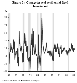
Residential investment is a highly volatile component of GDP. Yet as shown in Figure 1, the volatility has decreased markedly in recent years. Indeed, this series is one of the most frequently cited pieces of evidence when describing the overall decline in macroeconomic volatility (see Dynan, Elmendorf, and Sichel (2006) and Peek and Wilcox (2006)). Before the mid-1980s, residential investment was characterized by periods of extreme boom and then bust. The response of residential investment to the strong economy and robust house price appreciation since 1996 has been much more gradual, by comparison.
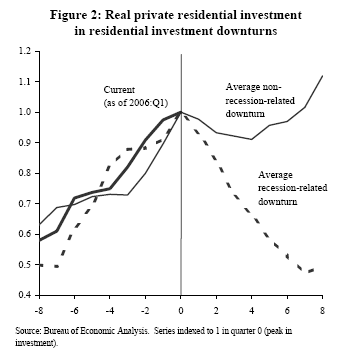 If we characterize an investment slowdown as two consecutive quarters of declining real spending, there have been eight downturns since 1976. The shaded recession bars in Figure 1 indicate that when the overall economy tips into recession, invariably residential investment turns down as well; however, the timing of these downturns does not always track the recession dates perfectly, and some downturns even occur during overall economic expansions. This leads to a natural classification of residential investment downturns. Recession-related downturns last an average of seven quarters and are characterized by large declines in investment; on average, real residential investment falls by about 50% from the previous peak (see Figure 2). These averages are strongly influenced by the downturns occurring before the 1980s, when the depth and duration of recessions were also severe. On the other hand, non-recession-related downturns are relatively shorter, lasting an average of two to three quarters, and relatively milder, resulting in an average dip in investment of roughly 10%.
Forecasting residential investment downturns
Residential investment should be thought of as the quantity of new housing supplied to the economy, and, in the long run, it should satisfy the overall demand for new housing. Thus, residential investment depends on supply factors, such as construction materials costs, as well as demand factors, such as demographics, interest rates (or the cost of capital), prices, and the stock of household wealth. These demand-side factors are particularly important in helping to explain why residential downturns tend to accompany economic downturns. In this spirit, a standard macro model of residential investment will typically posit that investment depends on variables like aggregate consumption, interest rates, and prices (see Brayton and Tinsley (1996)). Notably absent from this specification are the variables most cited in the press as evidence of a slowing housing market: sales volumes and growing inventories.
At any point in time, however, the new supply brought to market may not exactly equal the amount of new housing demanded. In particular, negative shocks to demand can result in there being too much supply on the market. If these changes in demand are not expected to be transitory, then developers will slow the pace of new construction and a downturn will occur. To forecast these turning points, we need to know what variables developers use to learn about changes in demand. It is possible that variables that do not enter into the model sketched out above, such as sales volumes and inventory levels, are related to the information that developers use to make, or alter, their plans.
In this type of framework, variables that speak to selling conditions for finished projects seem to be fairly useful in predicting downturns; for example, sales volumes dip one quarter before the average downturn in investment. For recession-related downturns, sales drop very quickly (by about 10%) once the downturn has started. For non-recession-related downturns, however, there is no clear signal, on average, from sales volumes data either before or during the downturn.
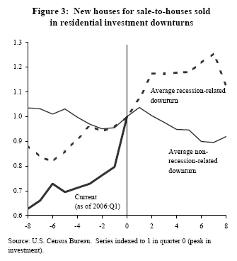 The so-called “month’s supply of housing” ratio, or the number of new housing units for sale in a given month divided by the number of new units sold, is also fairly useful for predicting investment downturns. For recession-related downturns, the ratio (shown in Figure 3) starts to rise on average six quarters before the actual downturn, and continues to rise for six quarters into the downturn. For the average non-recession-related downturn, the inventory ratio turns up just one quarter before the downturn and then eases back down after two quarters (which is also the average duration of a non-recession-related downturn).
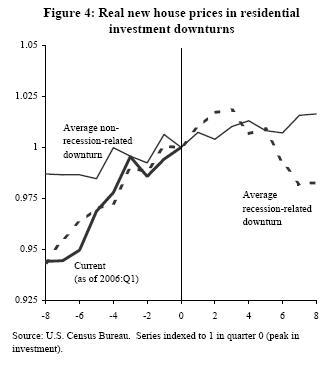
This exercise indicates that prices seem to be considerably less useful predictors of downturns than quantity-type measures. This might seem surprising because, unlike sales volumes and inventories, prices have a forward-looking aspect and thus would seem to be good predictors of the future state of the housing market. Figure 4 shows the average behavior of real new house prices leading up to and then following a peak in residential investment. The focus here is on new house prices because, presumably, they, rather than existing house prices, are most relevant for real estate developers’ decisionmaking. Additionally, new house prices are likely to be more sensitive to market weakness than existing house prices. Developers are always “motivated sellers.” If demand is soft, they generally do not have the option of withdrawing the house from the market and simply living in it. For recession-related downturns, the real price of new houses declines about four quarters after the peak, on average. Real new house prices register no detectable declines surrounding the average non-recession-related downturn. This basic stylized fact is even more apparent when using prices of existing homes. Only in the severest downturns do we witness real price declines, and never do these price declines come in advance of a downturn in investment.
 One caveat to this analysis is that it is based on the comparison of the average behavior of a housing market series leading up to two different types of downturns in residential investment. Obviously, averaging in the figures masks a fair degree of variation across the different downturns. However, more formal statistical modeling supports the notion that variables such as sales volumes and inventory ratios yield earlier and more reliable signals when the downturn is recession-related. This is natural; recession-related downturns have tended to be more severe than the non-recession-related episodes.
It is also interesting to note that the recent behavior of the month’s supply ratio bears more resemblance to the typical behavior before a recession-related downturn than to a non-recession-related downturn. Yet economists, such as those sampled in surveys of professional forecasters, are generally predicting only a moderation in overall economic growth in coming quarters. Given these conflicting observations, it is natural to wonder how much stand-alone information for predicting residential investment is contained in the housing market data. The answer, based on the last 30 years of data is mixed. If we estimate a model of the event that a residential downturn occurs using lagged values of the housing market variables mentioned above, we can generally improve the model prediction error by adding in forecasts of output growth. This suggests that it is best to consider economy-wide factors in addition to specific housing market variables when evaluating the real estate market.
Housing market statistics, such as sales volumes and months of supply on the market, can provide some useful information about turning points for residential investment. Much of this early warning, however, comes in advance of severe, recession-related downturns. Before non-recession-related downturns, which are typically relatively shorter and milder, these variables are less reliable. The analysis suggests that incoming information from the housing market should be evaluated in the context of the overall economy’s performance. To the extent that forecasts for solid output and employment growth are realized, this would not preclude slower growth in residential investment, but it should provide support for the real estate market and residential investment.
John Krainer
Economist
[URLs accessed June 2006.]
Brayton, F., and P. Tinsley, eds. 1996. “A Guide to FRB/US: A Macroeconomic Model of the United States.” Federal Reserve Board Finance and Economics Discussion Series.
Dynan, K., D. Elmendorf, and D. Sichel. 2006. “Can Financial Innovation Help to Explain the Reduced Volatility of Economic Activity?” Journal of Monetary Economics 53(1), pp. 123-150.
Peek, J., and J. Wilcox. 2006. “Housing, Credit Constraints, and Macro Stability: The Secondary Mortgage Market and Reduced Cyclicality of Residential Investment.” American Economic Review 96(2) (May), pp. 135-140.
Opinions expressed in FRBSF Economic Letter do not necessarily reflect the views of the management of the Federal Reserve Bank of San Francisco or of the Board of Governors of the Federal Reserve System. This publication is edited by Anita Todd and Karen Barnes. Permission to reprint portions of articles or whole articles must be obtained in writing. Please send editorial comments and requests for reprint permission to research.library@sf.frb.org