
The federal government routinely uses government spending and taxes to help offset the highs and lows of the U.S. business cycle. While government spending typically increases during a recession, the magnitude of the fiscal expansion during the pandemic recession was outsized compared with the average historical pattern. This likely contributed to real economic growth and possibly inflation during the recovery. Over the next few years, U.S. fiscal policy is expected to be roughly neutral, providing neither a tailwind nor headwind to the overall economy.
The stance of U.S. fiscal policy—whether it’s stimulating or slowing economic growth—has fluctuated greatly over the past 20 years. Some of this is to be expected given the large economic swings due to the Great Recession of 2007-09 and the pandemic. Yet, we show in this Economic Letter that the fluctuations were much larger than the typical cyclical patterns since 1960. Looking ahead, we conclude that fiscal policy is likely to be neither a headwind nor tailwind for economic growth over the next few years.
How does the primary deficit affect short-run growth?
According to traditional Keynesian economic theory, changes in fiscal policy can have important short-run effects on the macroeconomy. For instance, government spending on goods and services adds directly to economic growth as measured by GDP, which is defined as the sum of private-sector consumption and investment, net exports, and government consumption and investment. In addition, when the government increases spending through transfers to households and businesses, such as unemployment insurance payments or funds for food assistance, the recipients will spend some portion of that added money on goods and services, contributing to GDP. Government spending also has knock-on effects. When a household or firm spends more on goods and services, the firms producing those goods and services take in more income to share with owners, suppliers, and workers, who then have more to spend on other goods and services. The cumulative effect on GDP is known as the government spending multiplier.
Taxes work the same way but in reverse: tax increases reduce the amount of money that households and businesses have to spend on goods and services, at least in the short run. As with spending, tax changes have knock-on effects, and the cumulative effect on GDP is called the tax multiplier. Because government spending has a positive multiplier and taxes have a negative multiplier, the deficit, which equals spending minus tax revenue, has a positive multiplier. Economists generally focus on the primary deficit, which excludes the government’s interest payments on its debt.
A great deal of empirical research has focused on the size of the fiscal multiplier. Estimates vary widely, which largely reflects that in reality there is no single universal fiscal multiplier. The multiplier varies by context, such as whether the economy is in a recession or expansion and whether monetary policy is constrained by the zero lower bound on interest rates. A common central estimate is a fiscal multiplier of one, though some evidence suggests it is higher for tax-driven changes in the deficit than for spending-driven changes (Ramey 2019). A multiplier of one implies that an increase in the primary deficit equal to 1% of GDP raises GDP by 1%. Many economic forecasters draw on this simple logic to judge whether recent and projected changes in the primary deficit are a headwind or tailwind to near-term economic growth.
The multiplier concept also lies behind the rationale for short-run stabilization policies. Governments often use taxes and spending to help stabilize the economy through the peaks and troughs of the business cycle. They rely on two broad types of fiscal stabilization policies. The first is automatic stabilizers, which automatically alter tax revenue or spending in response to economic fluctuations. Examples include unemployment insurance (UI), which is normally available for six months to individuals who lose jobs; Medicaid, for which the number of qualifying households rises in recessions and falls in booms; and income taxation. The second type is discretionary stabilization policies, which are legislative actions taken by the government in response to current business cycle conditions. Examples include the tax rebates to households in the 2001 recession, the stimulus spending and temporary tax cuts in the 2009 American Recovery and Reinvestment Act, and the temporary enhancement and extension of UI benefits during the pandemic recession.
Stabilization policies in modern U.S. history have tied the federal primary deficit closely to the business cycle. Figure 1 compares the primary deficit (blue line) and the civilian unemployment rate (green line) from 1965 through 2022. When the unemployment rate rises and economic activity slows during recessions (gray bars), the primary deficit also rises. This cyclical pattern was especially pronounced in the two most recent recessions.
Figure 1
The cyclicality of the federal primary deficit
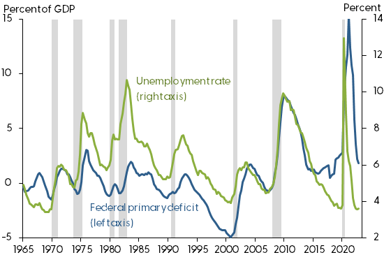
Note: Gray shading indicates NBER recession dates.
Source: Bureau of Labor Statistics and Bureau of Economic Analysis via Haver Analytics.
While state and local governments also contribute to the cyclicality of fiscal policy, their contribution is relatively small compared with the federal government. This is because nearly all state and local governments have balanced budget rules that greatly limit deficits being carried over from one year to the next.
Recent fiscal policy and historical trends
Given the strong cyclical behavior of federal fiscal policy, it’s not surprising that the federal primary deficit jumped during the pandemic recession. However, the magnitude of the jump was less predictable. To see this, it is useful to break the primary deficit into three components: the structural component, which captures the long-run average level and trend of the primary deficit; the normal cyclical component, which captures the average historical relationship between the business cycle and the deficit; and the excess cyclical component, which is the cyclical response beyond its average historical pattern. Note that the term “excess” simply conveys that it is above or below what average historical behavior would predict, based on a statistical analysis, and is not meant as a normative description. Following Lucking and Wilson (2012), we estimate the structural and normal cyclical components using a simple regression model and data from 1960–2022. We use a measure of the output gap, which is the percentage difference between actual GDP and potential GDP, from the Congressional Budget Office (CBO) to measure the business cycle. The structural component is captured by the constant and a linear time trend in the regression. The excess cyclical component is the residual of this regression—that is, the remaining portion of the deficit not explained by the first two components.
Figure 2 shows the total federal primary deficit (gray line) through the fiscal year ending in September 2023. Note that the 2023 value is preliminary as reported in CBO (2023); values for 2024 and beyond are CBO projections. The bars in the figure show our estimates of the annual contributions from structural (gold), normal cyclical (green), and excess cyclical (blue) components.
Figure 2
Federal primary deficit and its components
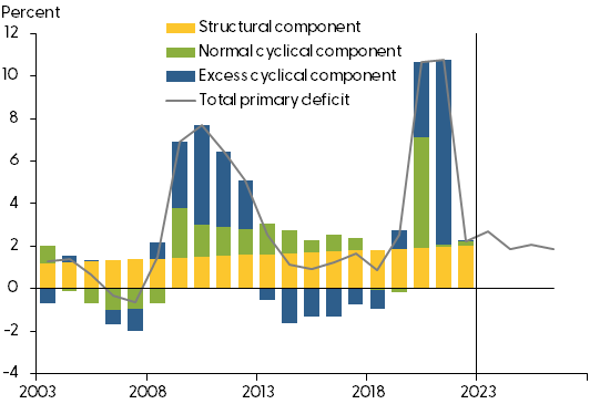
Note: Total primary deficit shows CBO projections beginning in 2024.
Source: BEA, CBO, and authors’ calculations.
The results show that the primary deficit’s increase during the pandemic recession was far larger than one would have expected given the average historical relationship between the output gap and the deficit. Specifically, given the sharp widening of the output gap in 2020, the average historical pattern would have predicted a primary deficit increase to around 7% of GDP. Instead, it rose to nearly 11%. This excess cyclical component was even larger in 2021. In that fiscal year, the output gap returned to roughly its historical average, hence the typical cyclical response would have been for the deficit to return to its historical average plus its long-run trend. Instead, it stayed at roughly 11% of GDP. It is worth noting that the cyclical response of the deficit was also higher than normal during the 2008–2009 recession and its slow recovery, though the fiscal response was more spread out over that period.
What accounts for the large increase in the deficit during the pandemic recession? Figure 3 shows what happened to federal revenue and primary spending (which excludes net interest outlays) over the past 20 years. During the pandemic, tax revenue as a share of GDP remained close to its historical average, while spending increased dramatically. As Figure 2 implies, this spending increase, especially in 2021, was largely the result of discretionary policy. In particular, several major spending bills, including the $2 trillion Coronavirus Aid, Relief, and Economic Security Act, were enacted over the course of 2020. These pieces of legislation included spending on small business support, unemployment benefits and other household transfers, aid to state and local governments, and health care. To be clear, this spending surge and the resulting “excess” cyclical response of the deficit do not say anything about whether this was good or bad policy. These calculations simply document how unusual fiscal policy was during this episode, which is perhaps not surprising given how unusual the pandemic recession itself was, being not just an economic crisis but also a health crisis. Nonetheless, the large increase in the deficit was likely a strong tailwind to stimulate economic growth during the pandemic recovery. Given supply constraints during this period, it may well have also contributed to inflation (see Jordà et al. 2022).
Figure 3
Federal primary spending and revenue
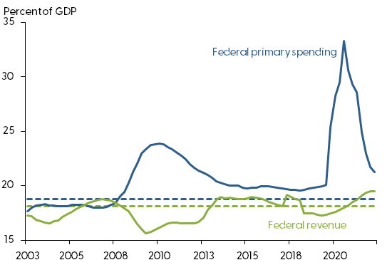
Note: Dashed lines indicate 1960–2022 averages.
Source: Congressional Budget Office and authors’ calculations.
Will near-term fiscal policy be a headwind or tailwind?
Recall that, according to the fiscal multiplier concept, increases in the deficit relative to GDP can boost economic growth in the short run, while decreases do the opposite. Looking ahead over the next few years, the federal primary deficit as a share of GDP is expected to be essentially flat. This can be seen in the CBO’s deficit projections for fiscal years 2024 to 2026 in Figure 2.
The small increase in the primary deficit in 2023 is projected to be followed by a small decline, which suggests that fiscal policy provided a modest tailwind to economic growth in 2023 but could be a small headwind to growth next year. Beyond 2024, the CBO projects that the deficit will be roughly flat, indicating a neutral fiscal stance that would be neither a tailwind nor a headwind for near-term economic growth.
Conclusion
Conventional macroeconomic theory states that fiscal policies that increase the primary deficit can boost short-run economic growth. This Letter finds that fiscal policy was unusually expansionary during the pandemic recession, which may have contributed to both real economic growth and inflation during the recovery. Over the next few years, the stance of fiscal policy is likely to be roughly neutral, providing neither a tailwind nor a headwind to near-term economic growth.
References
Congressional Budget Office. 2023. Monthly Budget Review: September 2023. Report, October 10.
Jordà, Òscar, Celeste Liu, Fernanda Nechio, and Fabian Rivera-Reyes. 2022. “Why Is U.S. Inflation Higher than in Other Countries?” FRBSF Economic Letter 2022-07 (March 28).
Lucking, Brian, and Daniel J. Wilson. 2012. “U.S. Fiscal Policy: Headwind or Tailwind?” FRBSF Economic Letter 2012-20 (July 2).
Ramey, Valerie. 2019. “Ten Years after the Financial Crisis: What Have We Learned from the Renaissance in Fiscal Research?” Journal of Economic Perspectives 33(2), pp. 89–114.
Opinions expressed in FRBSF Economic Letter do not necessarily reflect the views of the management of the Federal Reserve Bank of San Francisco or of the Board of Governors of the Federal Reserve System. This publication is edited by Anita Todd and Karen Barnes. Permission to reprint portions of articles or whole articles must be obtained in writing. Please send editorial comments and requests for reprint permission to research.library@sf.frb.org