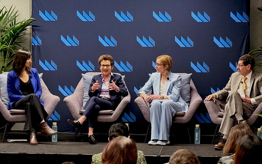
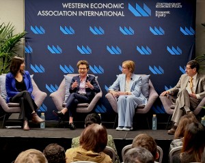
James H. Stock, Harvard University The Macroeconomic Impact of Europe’s Carbon Taxes

Date

Thursday, July 16, 2020

Time

SF 8:00am, NYC 11:00am, BERLIN 5:00pm

Location

Virtual

James H. Stock is the Harold Hitchings Burbank Professor of Political Economy, Faculty of Arts and Sciences and member of the faculty at the Harvard Kennedy School. He received a M.S. in statistics and a Ph.D. in economics from the University of California, Berkeley. His research areas are empirical macroeconomics, monetary policy, econometric methods, and energy and environmental policy.

Download the paper (pdf, 2 mb)
Download the slides (pdf, 3 mb)


Seminar and Q&A recording (video, 55:43 minutes)

Transcript

Hide this section

James H. Stock:

Today, I’m going to take the opportunity as the first speaker in this series to make a few comments that are very high-level to just lay out some of the overall challenges and then I’m going to turn to the paper at hand. The paper at hand is with Gib Metcalf, so let me get started with my slides here. The paper at hand is some work that I’ve been doing with Gib Metcalf on the macro impacts of carbon taxes, but I want to start at a higher level. And I think actually I’m going to start with this picture. That is your picture for the climate seminar and talk about that a little bit. So you have plotted here for all of us, for many on the call, they will recognize this as a time series of annual temperatures that are of our global temperatures. And so I’ve just reproduced a slide from another talk I gave of a time series of global temperatures. And the reason I’m reproducing this, is that it actually has a very simple regression in the background. The very simple regression in the background is one that relates temperature to what’s called radiative forcing, which is the amount of energy forced back from the atmosphere associated with and incoming on the Earth’s surface, combination of insulation and then in particular, the greenhouse gas re-radiation emissions, also cooling from atmospheric sulfates. So what you have here in the red line is the predictive value. The model actually was fit back to like 1998 or something like that. So these are out of sample predictions. The important part of this is that at one point, and I think this has been diminished quite a bit, but at one point there was a debate about how much of warming is anthropogenic. What this very simple model does in a way that’s way simpler than the actual fancy climate models. So it allows you to do that decomposition into part that is natural and so it’s just a natural emissions component on solar insulation and then everything else. And you can basically see that the natural fluctuations are stationary and small and the everything else component is the anthropogenic component and that is large and growing, so the problem is substantial. Solving this problem requires in the first instance, reducing anthropogenic emissions of greenhouse gases. In United States, these greenhouse gas emissions peaked in around 2005, and then they’ve been declining since then. And so a lot of people view that as optimistic and indeed it is, this is good news. We have a target, or we had a target associated with the Paris agreement, which we have left, but that target had us at about a 27% reduction by 2025 below the 2005 levels. And, you know, roughly speaking, we have been in that vicinity. That is associated to a considerable extent with the switch from coal for generation of electricity, to renewables and natural gas, which are lower emissions, lower or zero emissions. And so that’s good news. I think that it’s important to remember that there’s a lot of work ahead of us. Not only do emissions remain high, but if you look at projections from, for example, the U..S Energy Information Administration, you see that those emissions reductions will be plateauing. After all, there’s only so much coal that we can drive out and while remaining have a lot of natural gas and still be driving petroleum-based automobiles, and at least according to the EIA projections as of January, they have emissions growing under current policy out into the 2030s and 2040s. Needless to say, this is not the direction that we need to be going. It’s also I think a noteworthy thing to look at and maybe something that we’re not always familiar with or have in the front of our mind is how much generation we actually have, how much penetration there actually has been by wind and solar. This is generation in the United States, electricity generation in the United States as a fraction of total generation or percent of total generation and generation by gas is in the lead with 38% and coal used to be in the lead, but isn’t anymore. It’s been driven out mainly by cheap natural gas. More recently, it’s been driven out by wind and by solar, but what’s really striking and I think should be striking about these percentages right here is that wind and solar combined are less than 10% of generation in 2019. Hydro isn’t going be increasing because we’re not going to be damming a lot more rivers. Nuclear, if anything, is going to be decreasing because of retirement of existing nuclear plants. So even within the power sector, the challenge ahead of us is very large. Because of carbon externalities, because of investment externalities, because of network externalities, chicken and egg externalities, like having EV charging stations, the market’s not going to take care of this on its own. So these are all issues that require policy interventions. Today what I’m going to do is I’m going to talk about the policy tool that’s loved by economists, which is a carbon tax. And so let me turn to that. Let me turn to that particular topic. So a carbon tax is something that’s been proposed for a long time, been discussed among economists for a long time. It’s gaining additional traction in both the sort of the public intellectual sphere and also in Congress. There are a number of bills that were introduced this year for a carbon tax. And so this is work from the Columbia Center for Global Energy Policy that has plotted out the tax rates associated with these different bills. It’s something that I’m sure many of you are familiar with as being pushed by the Climate Leadership Council, which has proposed a specific carbon tax plan with a dividend, a rebate. So you take the dividends and then you distribute them more or less evenly across the population. So that has a fair amount of political economy appeal at least, and would also introduce a price on carbon. So, these are proposals for the United States. These are proposals for the United States. They are not without controversy. So here’s some particular statements about the Paris Accord. So the Paris Accord, when the Trump administration pulled out of the Paris Accord, they issued a statement that said that sticking with the Paris Accord would lose 22.7 million jobs by 2025 and would result in $3 trillion in lost GDP. $3 trillion in lost GDP is… That’s a lot, that’s as much as we’re losing in the current COVID crisis recession, and 6.5 million industrial jobs. Now I’m not going to actually argue with these specific numbers. This NERA study is not something that I would take at all seriously, but the point is the framing. The framing is that taking actions to address climate change will cost jobs and will result in lower levels of GDP. So what we’re going to focus on is we’re going to focus on the impacts of a carbon tax on three things. First on GDP, second on jobs, employment, and third on emissions, which of course is one of the main, the main point of implementing a carbon tax. Well, it’s useful to think about what theory suggests in terms of what a carbon tax might actually do. So there’s been quite a bit of work using computable general equilibrium models and things of that ilk. Here’s one that’s a current one that’s available on the resources for the future website. There’s actually a cool little carbon calculator. And if I were a little bit braver with Zoom, I would take you there and we would do a simulation, but I worry that if I went there, we’d go to my email instead, and then I would never get back and we’d get quite derailed. So you can do this on your own, go and play with the carbon tax calculator. And you can say, well, I want to have a tax rate of this much that increases in this amount of revenue recycling of this amount and you’ll see some scenarios. I’ve printed out one of these scenarios or captured one of these scenarios. And what you can see is that the carbon pricing calculator, it works with a computable general equilibrium model, which is described in a Goulder and Hafstead book, but it has a long lineage. And what it does is, it says, well, by implementing a carbon tax, we’re going to be changing relative prices we’re going to be mak
ing people do something that they didn’t necessarily want to do. That’s imposing some costs on the economy. How big are those costs? And they’re not particularly big. So they estimate that over 40 years, for example, if you have, excuse me, if you have a $40 per ton carbon tax increasing at 5% per year, then by 2035, you will have lost, depending upon how you recycle the revenue, maybe one and a half percent of GDP and that’s if you do a dividend, like the Climate Leadership Council proposal. If you do a payroll tax cut, that’s a little bit more beneficial because you’re actually reducing a bad tax and you’re replacing it with a good tax and you get a small double dividend. It doesn’t quite pay for it, but these are pretty small effects. There may be a 1% or one and a half percent gap in GDP, a loss in the level of GDP, a decline in the level of GDP, as a result of the carbon tax Underlying these, I’m going to come back to this in our empirical work. Underlying these is, in the end, what asymptotes out here is that there’s a parallel shift. So the level of GDP shifts down, but the growth rate paths are parallel. And I’m going to refer to that as the parallel path assumption. We’ll be able to test that parallel path assumption, at least in a, you know, some sort of moderate, medium run using the European data. We will not reject it. In fact, it’s going to be consistent with the data that there is a parallel path shift. It turns out that in our empirical analysis, the parallel path shift is like zero or maybe positive as opposed to negative. But, but we do support the parallel path shift. More recent work by Hafstead and Williams has looked at employment affects. And so that depends how you model it. There’s going to be some friction because of course you impose a carbon tax on a sector that’s producing electricity, your carbon-intensive sectors, you’re going to be changing relative prices so that means the demand for labor in that sector is going to change. People are going to shift so that people become unemployed in one sector, but then they find a new job in another sector. And when you look at the whole overall shift, you end up seeing that there’s a hit to employment. In their particular calibration, hit to employment occurs pretty quickly. There is no anticipatory effects built in. The frictions are such that the shifts in employment occur pretty quickly, but there’s going to be some employment effect because you’re changing relative prices and therefore you’re changing demand for labor. I’m going to take a look at that too. So that’s a theoretical prediction using modifications of CGE models. We’re going to take a look at that up here. There are other frameworks for doing this. IAMS, Integrated Assessment Models, National Energy Modeling System, which is the EIA system, EIA model. The EIA model, NEMS, has a very, very detailed energy modeling sector. Its macro sector is not sort of very current. So I don’t really take it, put a lot of weight on the macro components coming out of those models, although there’s probably reasons to think that they do pretty good estimates on the actual energy response and emissions response to some interventions like carbon taxes. Okay, and so there’s a survey of this work in a recent Brookings paper by Gib Metcalf, my coauthor on this project. Okay, so I’m not going to go through this. Here’s the obligatory slide with a bunch of names on it. And some members of this audience have probably written a paper that doesn’t appear there and that’s my bad, and I apologize for that. There’s a fair amount of work looking at the effect of carbon taxes on emissions. And that’s part of this project. There’s actually quite a bit less work looking at the empirical effect, as opposed to the theoretical effect of carbon taxes on GDP and employment. And that is what we will do mainly here. So we’re going to look at evidence from Europe and there’s a variety of countries in Europe that actually have imposed a carbon tax. That European data is going to be the countries in the European emissions trading system, 15 of which have a carbon tax. Glenn, we were going to maybe pause here, see if there’s any questions. How are we doing? If you have questions, throw them up in chat and get Glenn to jump in.

Glenn Rudebusch:

Jim, right now we have no questions. You’ve been completely clear, for some reason.

James:

The latter does not necessarily follow from the former.

Glenn:

I do have someone asking, are you looking at agent-based models?

James:

Agent-based models, agent-base models, so that reminds me of my COVID epidemiological modeling and SIR models. We are not looking at agent-based models here. So the tools we’re going to be using here are going to be… My understanding is that many of the people on this webinar are from the Fed, so they’re kind of used to thinking about macro time series stuff and so I think maybe one of the reasons Glenn chose this, not quite sure, is that we’re going to start off with a familiar tool box, which is going to be a bunch of macro time series approaches to macro data. So that’s the framework we’re going to be using.

Glenn:

Another question is do the carbon taxes interact with the ETS?

James:

Yeah, so that’s a great question. Okay, so the scope of the carbon taxes… so that’s a great question. Let me pause on that for a second.

Glenn:

Maybe remind people what the ETS is.

James:

Yeah, okay, so the ETS, is the European Emissions Trading System. So it kicked off in 2005 and covers the power sector and some energy-intensive industries. It’s expanded to include aviation and some other smaller sectors, smaller components as well. So it’s been changing over time. Carbon taxes in some of these countries did initially include power sector, but then once the ETS came in, they scaled back. There’s one exception where there’s a complicated top-off scheme, which I suspect I won’t get right for the UK where the UK does ETS and then ups that to a carbon tax level. With that exception, the carbon taxes that we’re going to be looking at after the ETS cover only non-ETS coverage sectors, so that’s going to be primarily transportation. The coverage differs from country to country. Most of them cover the transportation sector. Some of them cover some heating components and so forth. So the coverage has changed over time and there is this interaction. We are going to include to take into account all of those complications, all of our regressions are going to have time effects and they’re also going to have country effects. So that’s going to help deal with some of that. And because all of the countries in the ETS are in this, all of the countries we use are in the ETS, we’re going to be having that essentially as a background state of control, where we’re looking at the marginal or additional effects of the carbon tax on top of the ETS. The short way to say that is basically, you should think about these carbon taxes as hitting the transportation sector.

Glenn:

Great, and so one way to summarize it would be is the identifying variation coming from the level of the carbon tax and the coverage?

James:

Yeah, so that’s right, so it’s coming from the level of the carbon tax and the coverage, and actually, these models were all identified in the time series. So we can estimate each one of these regressions, using time series data. Since it’s annual data and we only have data since 1985, you’re going to get pretty crummy standard errors, but it’s all identified in the time series and then we’re using the cross section to get additional variation.

Glenn:

Excellent. Okay. Thanks, Jim.

James:

Okay, so here’s our data sources. We’re using a new dataset from the World Bank on carbon pricing data. You can read the paper about it. You gotta do the sort of the usual things of figuring them out in local currency, converting them to U.S. dollars. We do that using a PPP. There’s a little bit of some complications about when you have multiple tax rates. We handle it in one way, which is we look at the fuel taxes, which are the ones that have the highest rates and also have the highest coverage. There’s some different ways you could… that’s not the only decision you could make. There’s an alternative dataset that Jeffrey Dolphin and coauthors have constructed. And they’ve generously shared that with us. And we’ve used their data too and you get very, very similar results, using some different judgements about how to construct the taxes. Both theirs and ours are weighted for coverage of the taxes. And you’ll see that that’s important because the coverage varies a lot by country. Using World Bank GDP data, population data, except for Norway, Norway has this really big oil and gas sector, so we’re using what they call mainland GDP, which is from Statistics Norway, and Ireland, Ireland is a great outlier. It turns out that five years after you implement a carbon tax, you have a giant boom in GDP, assuming that Apple transfers a great deal of intellectual property to you. And so there was, if you recall your GDP or Ireland GDP anecdotes, you will know what I’m talking about. So we don’t use those data. We use the Irish GDP data that are adjusted or GDI data that are adjusted for, to take out this Apple transfer effect. Okay, and then we’re going to look at emissions and we look at it here either in emissions not in the power sector, because we’re looking at the sectors that are affected by the carbon tax and we have two different ways to do that, either from total fuel consumption or from just these other sectors. So we’ll look at it a couple of different ways. Here’s the data. What we could do is we’ve got coverage and tax rates and I love the first two lines. There are two countries that started off early, 1990. Finland started off early, and by 2018, they have a $71 per ton carbon tax. That’s a pretty big number and covers about a little more than a third of carbon emissions are covered. Of course, the power sector is excluded from this. On the other hand, Poland started off in 1990. It has a 16 cent per ton carbon tax and it covers 4% of emissions. So there’s a fair amount of exogeneity here. And you can see some of them are actually quite high. So Sweden’s tax is really quite high, covering 40% of emissions.

Glenn:

How does this interact with the gasoline tax? You just somehow make that distinction?

James:

So, yeah, so we looked at this in a couple of different ways. In the end, all the regressions I’m going to show you here are going to be just separating out the carbon tax. So we’re just going to be looking at the effect of the carbon tax. There’s a couple of different ways that you could do it. You could roll in all energy taxes, or you could look at actually gasoline prices or the surcharge on top of gasoline prices. So you can model this in a number of different ways. If you look at it in terms of all taxes, you get basically the same answers here. It’s a little more delicate if you look at it in terms of the total gasoline price with this upped and that’s because then you’ve actually got gasoline prices and therefore oil prices on the right-hand side of the regression. And all of a sudden, you’re doing a bunch of other things too, in the macroeconomics. So we’re going to keep it as clean as possible, and just look at the carbon tax effects.

Man:

Jim, there is a tax per ton of carbon or tax per ton of CO2?

James:

Tax, so I might have misspoken. And if I said per carbon, I’m wrong on that. This is the usual units is tax per ton of CO2. Okay, so here’s just some pictures of the carbon taxes. You can see some of them started early, some of them have gone up. It’s interesting if you think about those schedules in that first picture, if you think about the schedule here, this schedule right here makes everything look nice and predictable and so forth. And we think of a carbon tax as being something that’s great because there’s a lot of predictability in a carbon tax, and it’s differentiated from cap and trade where there’s a lot of variability in prices. It’s kind of interesting just looking at the historical series here. And although some of them have been rising predictably, there’s other ones that, you know, there’s a lot of changes in the tax rates that maybe are not predictable as one might think. We’re going to be exploiting that predictability. So this is just an event study that looks at GDP growth before and after the imposition of a carbon tax. You really can’t see very much. These are the usual 95% event study bands, and you really can’t see very much here. I want to stress that we’re not actually going to be getting much identification from the before/after experiment. We’re getting variation from changes in the carbon tax rate. One of them occurs when it’s imposed, but we’re actually looking at all of the changes in the carbon tax rate so this is just illustrative. Similarly, these are what happens with employment growth before and after the imposition. It actually looks like there’s a slight increase, but it’s not statistically significant. And this is what happens with emissions before and after the imposition. You can see that in some countries, there may be some emissions decline prior to the carbon tax, suggesting that maybe other things are going on as well. We’ll want to be able to deal with that in the econometrics, but that’s not universally the case. There seems to be some emissions decline around the imposition date, but these are all just sort of starting points. Okay, let me talk a little bit about the methods. The simplest thing you might think about doing is just running a distributive line.

Glenn:

Here’s a question from Ravi Bonsal. I’m going to allow him to ask it.

Ravi Bonsal:

Hi James. So one question I had is you showed this time series of these various taxes. I wonder, and I fear that these are endogenous choices made by governments at different points in time. There’s so much variation. And if I look at the graph you had about the different countries and their coverage and the tax rate is seemed there is some, you know, like a Northern European cluster over there, and then there’s a European cluster, so on and so forth. So it seems to me it’s very endogenous. And so varying the tax rates at different points in time, and then thinking about the GDP response, I’m not sure if that answers the question or not.

James:

That is a terrific question. So that is exactly why you don’t want to use the first of these specifications. So the first of these specifications is you just run a regression of GDP growth on some control variables and on the tax rate. And the problem is exactly the problem that you indicated, which is the exogeneity condition there. Unless you’ve got all the control variables you need is going to be one where you assume that there has to be no feedback from past values of GDP to future values of the tax rates. So this is a strict exogeneity condition, conditional on the control variables, conditional meaning dependence condition. I don’t think that we would think that that would hold for exactly the reasons that you indicate. So that’s not what we’re going to do, okay? So what we are going to do, indeed, this is actually testable, and if you test it, I’m not going to bother to present that. That’s in the paper. If you test these restrictions, they’re rejected. What we are going to do is we’re going to rate a timing assumption and that timing assumption is that, and combined with fixed effects. So first of all, we’re going to include country fixed effects. So that might go some direction towards the Northern European and Southern European, for example. Second thing we’re going to do is we’re going to include year effects. So that is going go some direction towards like there’s a global financial crisis and as a result of the global financial crisis, we might be changing carbon taxes. And the final thing that we’re going to do is going to be including lagged values of GDP, as well as the fixed effects. The W’s are the fixed effects, as predictors. And so then there’s a couple of different ways to say what the exogeneity that we’d be needing is this is sort of the formal statement, which is that conditional on the past values of the tax rate and past and current and past values of GDP and the control variables or the fixed effects that the mean of the error term no longer depends on the current tax rate. You know, timing conditions have a long history in macro, and you always kind of wonder, like, you know, can the Fed change something in the interim or something like that? Here for carbon tax rate, I think I have a certain degree of comfort with this. And the reason is that these rates have to be determined the year in advance. These rates, you know, you publish the carbon tax rate schedule for the coming year, or maybe the coming fiscal year and you’re going to publish that in a way that then people can actually implement if it gets built into the fuel prices and so forth. So the concept of current shocks, the unpredictable component of current shocks affecting the current carbon tax rate, I think assuming that that doesn’t happen seems to me to be a reasonable assumption. We can discuss that, but in this world of timing restrictions, especially since we’re conditioning, we have year fixed effects in here, I think I’m willing to defend that. And you can implement that both by local projections and by panel VARs. So the panel VAR has exactly the same identifying assumptions, same conditions for . All right, so there’s two flavors of this that we do. Remember the parallel paths assumption. The parallel paths assumption has parallel paths, which is that, in the long run, the growth rate is going to be the same. The growth rate of GDP is the same. There’s just going to be this downward shift. That’s a testable hypothesis and the parallel paths assumption might not be true. There might be an effect of the level of a carbon tax on the longterm growth rate of GDP and we’re going to be able to test that assumption. It turns out that that assumption is not rejected. Okay, let’s see, did I say everything here? Oh, yeah, all of the calculations are going to be for a $40 carbon tax. And just to make it simple, we’re going to have a 0% real increase. Because we only have a fairly short amount of data, we can’t do a simulation out to 2050. We’re going to look at impacts over the next, like six or seven years. To do this counterfactual, not using like a standard deviation shock, but a shock is calibrated to a $40 carbon tax, we’re going to use the method of backing off what the shocks to the carbon tax would need to be to implement that. But since the carbon tax is a highly persistent process, it’s basically just this one time innovation. Okay, four lag, so let me look at some, oh here’s-

Glenn:

Jim, one more.

James:

Yeah, sure, sure.

Glenn:

From Rich Entel, so if the effective tax rate is the nominal tax rate times sectoral coverage, that’s kind of a definition of the effective tax. That assumes the tax would have a homogeneous effect on economic sectors and that policy makers randomly selected sectors to be taxed. Is that…

James:

You know, you could look at it that way, or you could say maybe it’s really complicated and I’m going to take a first-order Taylor series expansion, and only the first term is anything that I have a prayer of identifying. So that’s a great question for future research.

Glenn:

Excellent, thank you. I’ve got one more-

James:

It’s a great question, that’s a great question. You know, you could add different triangles in different sectors. It’s a good question.

Glenn:

I’ve got another. Ravi Bonsal has another question to ask.

Ravi:

James, I’m still a little bit unclear as to why would you ever expect the response from these taxes on output after you do all the controls and restrict the response of growth rates, why would it ever go positive? Is there like an economic reason to think about that or should you be imposing a constraint on that as well?

James:

You know, I don’t know. Like, I don’t know, what’s the right way? I don’t want to be… Oh, what’s the right way to phrase this? I think if you listen to certain elements of the policy debate around the energy transition, they have positive signs on their transition effects, so I’m just looking at-

Ravi:

Which the free market doesn’t adopt.

James:

We’ll look at the empirical estimates. I take the point, I take the point for sure. Let’s look at, the standard errors are going to be around zero so let’s just look at the results. I take the point. Okay, here’s the parallel paths restriction assumption. It’s probably not worth staring at these. The bottom row of each of these, which should have parentheses around it, these are all P values and you can use an either LP or SVAR estimates and none of these P values suggest that there’s really any rejection. I’m going to look at results that are going to have both the parallel path assumption imposed, which is what the CGE model theory suggests, and ones that relax it. They’re going to look really similar. And the reason they look really similar is because the longer term effects are small enough not to be significant. Okay, so here’s an example. So let’s do some results. So this is an impulse response function. So what we’re looking at here is we’re looking at our full dataset, which is these 31 countries. We’re using linear projections. Unrestricted means that we do not impose the parallel path assumption. So we’re allowing a long-term effect of the level of a carbon tax on the growth rate of GDP. That’s not statistically significantly different from zero, but this is the unrestricted version of it. We have year effects and we have time effects and we’re using this share-weighted carbon tax and what you can see, there are so we have one and two standard deviators, so 67% and 95% confidence intervals here. And what you can see is that the confidence interval, there’s this slight positive point estimate of the growth rate. That said, you know, they’re not more than one standard error away from zero throughout this entire thing, so I certainly wouldn’t push for this being a positive effect, but what it is is it’s not a particular negative effect. It’s I think a reasonable interpretation of this would be essentially no effect on GDP growth. You can look at the SVAR, so now I’ve got to do something. I have far too many slides here for a short talk, but I just couldn’t help but nerd out on the SVAR LP thing. For those of you, and I know Oscar is one of the participants here, we just have said so many arguments and one time series seminar versus another time series seminar over SVAR and LP and getting different results and a what should you use, I just want to show some of the coolest results. This is the LP result, and this is the SVAR result. And again and again and again, so here it is for the restricted version of the LP and the restricted version of the SVAR. It’s actually just unbelievable. So look at this dark red line. That’s the central point. That’s the point estimate, that’s the LP estimate, and this is the SV estimate, that’s the SVAR estimate. It’s like, they’re the same. This never happens. You never get LP and SVAR estimates are the same. And I think that this is just an indication of having the additional degrees of freedom with the cross sectional estimates, to just get rid of the noise. Theory and population, these guys should be the same and we’re seeing that they’re actually the same in sample again and again, in this exercise, which is great fun. It happens to be that the LP estimates and these data happened to have smaller standard errors. Okay, anyway, this was the restricted version. When you restrict the long run effect to be zero, remember that’s not rejected. You see that it’s basically just zero. We’re just getting no effect on GDP growth. Same thing in SVAR. If this is a cumulative impact, if you were restricted the long-term effect would be the parallel paths assumption. This is the cumulative impulse response function. So now this is the departure of the level of GDP from the hypothetical, no tax baseline for a $40 carbon tax. Remember how the CGE model had you going a little bit down. So you were a little bit unhappy and you lost a little bit of output because you were making the shift in relative prices. Well, you see a tiny little, certainly not even remotely statistically significant increase, and then in the cumulative effect after six years, it’s zero, it’s just zero. This is the SVAR estimate, which is also zero, just a little bit noisier. Okay, what about employment? So this is the employment estimate. For reasons that are not quite clear in the data, there seems to be a little bit of an initial boost in the growth rate of employment, but that then dissipates. And it certainly, again, is not statistically significant and then has no long run effect. That’s true in the SVARs. Here’s another, just like amazing pair of SVAR LP results. Let’s see, this is restricted so this is imposing zero long-term effect. Okay, manufacturing employment, be kind of interesting to see whether there’s specific sectoral effects, like you’d think maybe manufacturing would be hurt by this. It just turns out that’s too noisy so we can’t really say anything. So that’s the manufacturing. Emissions, so you’d think that they’d reduce emissions and what you estimate is in fact, there is a reduction in emissions. These are the cumulative impulse response functions for a $40 carbon tax on its effect on emissions. Reduces the level of emissions on impact and then it continues to reduce it a little bit more so that’s maybe down 4% or so by the end of six years for a $40 carbon tax. This is the cumulative impulse response using LP and the restricted case parallel paths assumption. This is the SVAR version, which gives you basically the same estimates, but it’s just not as precise. Okay, let’s see.

Glenn:

Jim, do you want to take a… I’ve got a few more.

James:

Yeah, so let me just, this is the final slide and this is just, that was emissions on the carbon tax affected sector. It’s just a robustness thing, is using emissions fuel consumption. That’s not quite as crisp because that includes some power sector stuff too. Okay, some questions, yes.

Glenn:

Let me unmute Rene Ramos.

Rene Ramos:

Hi there, thanks James. My question really is, you know, at what point of carbon tax do you start seeing that the parallel hypothesis fails?

James:

Yeah, so that’s a great question. So let me go back up to, for example, this GDP growth one, which is the cumulative impulse response function. Okay, so how we’ve calculated this to a first approximation is you basically compute the shock to a carbon tax that is necessary to give you a $40 carbon tax. So you figure out what that shock is. And then you just compute the dynamic response to that. That’s true of first approximation. That’s not exactly right, because we have to compute a few additional shocks down the road. The T statistics and F statistics are all going to be invariant to the magnitude of that shock. Is it a $40? Is it a $60? Is it $120 shock? And the reason for that is that this is a purely linear system. We tried estimating early on in this exercise, some nonlinear things, well, gosh, maybe a $10, or $20, or $30 carbon tax is going to have a negligible effect, but you might be damaging the economy more than linearly from $120 carbon tax. So that’s a really interesting, it seems like that’s a great question. Not surprisingly, for those of you who work with macro data, you can’t tease that out of the data. So that’s a standard error. It’s just become so big that you can’t really say anything, even though it’s a tempting thing to look at. So we can’t answer that question in these data. What we can say is that for carbon taxes in the range that have been tried, you know, on average in the middle of that range, the usual linearity type assumptions, it seems to be essentially a zero effect and no departure from this parallel, and not just a parallel path, but the same path.

Glenn:

Jim, and then there are several questions about thinking about the positive effects so Rob Engle asks because climate damages are due to an externality, a carbon tax would have a positive effect on social welfare. This might encourage investment in consumption. Hence, positive shifts could be justified.

James:

Yes, yeah, so I mean, to be clear, GDP is not welfare. So, you know, the reason you do a carbon tax is because it’s improving longterm present value welfare. GDP isn’t welfare. You know, I don’t want to over-interpret. I don’t want to over-interpret this positive effect right here, which is approximately a third of a standard error away from zero. So I’m going to just stick with zero.

Glenn:

Okay. There was a question from Phillipe Hellman, does the macroeconomic impact of a carbon tax, it should depend on the mode of recycling its revenues. Are there differences in recycling modes across the countries in the sample?

James:

That is like, I love these questions. So that is question one on the next slide, which is, and does it depend on how we recycle the revenue? So that is terrific. And we actually can take a look at that here, because we have essentially almost a partition of the carbon tax countries into two groups. So there’s a group that said, we’re going to use this. We’re very explicit. We’re using this to reduce marginal tax rates. And that’s like the Scandinavian countries, plus Switzerland and Portugal. This was part of an overall tax reform to substitute good taxes for bad taxes. And then the rest of the countries it’s basically just goes into the general coffers. So it’s almost a complete partition. Not quite, I think Switzerland was 67% offset, but everybody else was 100% offset or 0% offset. If we just restrict the sample to the revenue recycling crowd, and this is LP using restricted, you know, you see this positive effect on GDP here initially, maybe a little bit of a negative effect, and then it comes out. And if you think about the cumulative effect, you’re going to be adding some positives and some negatives. And so it’s basically zero. So, and everything is within, you know, two standard errors of zero. So, you know, we had sort of thought that like, maybe you’d see, it would be really great if you would see this one like way, way up here and then the next one would be way down here and then that would be like a very cool result, but it’s just sorta noise. So we can’t, we don’t have, again, this is just one, it’s a great question. This is the non-revenue recycling countries and there’s just not enough precision. So there’s a partition of revenue recycling and non-revenue recycling countries, but I don’t think you can say anything, unfortunately.

Glenn:

Jim, we also have had some questions about anticipation, I’m going to let Dan Wilson ask his question about anticipation.

James:

Yeah.

Glenn:

Dan, you’ve got to unmute.

Dan Wilson:

Okay, can you hear me?

James:

Yeah, please.

Dan:

Okay, great, thank you. Yeah, so related to the earlier discussion about the timing in identifying restrictions. So I understand the logic that current GDP growth shouldn’t affect current tax rates, but I’m wondering about anticipation effects. And so the methodology here seems very reminiscent to me of the fiscal multiplier literature. the timing assumptions there when looking at tax or spending multipliers and there, you know, Raimi and others have emphasized the importance of the timing anticipation effect. And so I think this concern seems particularly acute when thinking about the dependent variable being emissions. And so in particular, it seems quite plausible that the transportation sector businesses would be starting to alter their emissions in anticipation of upcoming carbon tax adoptions or rate changes. So, you know, how have you thought about that?

James:

So that’s an excellent question. So just want to rephrase what the identification here is. So, because we have lag values of the carbon tax and lag values of GDP and country effects and time effects, but forget about those latter ones on the right hand side, just by sort of , the identification is the unanticipated component of the carbon tax affecting the unanticipated component and subsequent unanticipated components of GDP. Now, you know, one could argue that this is just a linear approximation and maybe some nonlinear schedule might give you a better sense of what those unanticipated components might be artifacts. And I would get. This is living within a linear linear approximation, which is all we can probably hope to identify a thing. But I do take that point. If you think that really what the carbon tax is doing is it’s providing a signal, or is part of a package or part of a general shift towards lower carbon emissions in the transportation sector, I guess you’d be picking up some of that in the fixed effect, averaging it out. But I think I’d have to think harder about how… That wouldn’t be picked up in this identification scheme I don’t think, because here this is these unanticipated components. So I think that the question you raise is an important one, but given the frequency that we’re looking at, we’re actually not going to be picking that up. So you could argue that our reductions are too small because we wouldn’t be picking up that effect.

Dan:

Right.

Glenn:

Jim, on this point, not particularly this slide, but some of your slides suggested that there was an immediate effect of the carbon tax. Richard Cole asked this question. Immediate effect of the carbon tax and it stayed the same over several years. Again, not for this slide, but many of your earlier slides. And so the tax applies mostly to transport emissions and does this suggest that the response is behavioral rather than capital replacement or technological change? You’ve got this immediate effect that stays fairly-

James:

Yeah, I think that’s the way I would interpret it. I mean, you know, I think, I guess I wouldn’t, this is all linear, it’s all annual. So I would not overthink this. I would think, “Oh shoot, the price of gasoline has gone up. I guess I’m going to drive just a little bit less or maybe I’ll, you know, use my other better fuel economy car a little bit more.” And you’re just seeing a shift along the demand curve, which in the first instance is the first thing that you would expect in a carbon tax that is affecting fuel prices.

Glenn:

That’s great. We’re going to let you finish your presentation now, and then we’ll have some questions at the end.

James:

Okay, that’s great, so I think we got the main points of the pictures and yes, I understand these sort of persistent things. What I would stress is that basically all of these things, certainly the GDP and employment ones are pretty much within a standard error of zero. Okay, so a couple of comments, I think some good comments have come up and maybe people can, I’m going to give you some other talking points here, if you want to criticize the paper, but let me just shift to the bigger picture. So these were small effects. So the conclusion is should we, you know, was the White House right to pull out, you know, when they said that climate policy is going to devastate the economy? Well, if it’s a carbon tax of $40 a ton affecting their transportation sector, the answer is no. Is anyone right if they say that a carbon tax of $40 a ton affecting the economy is going to transform our CO2 emissions and drive them to zero? Well, again, the answer is no. That’s 40 cents a gallon. Again, price, last time I checked this morning, it was like 2.20 a gallon. So that would bring it up to 2.60 a gallon. And that’s going to have some effect on behavior and some effect on consumption, but it ain’t going to have much effect on consumption and behavior. So, if I step back, you know, yes, for sure, a carbon tax is a very important component, getting a price on carbon is an important component of climate policy. Getting one that’s big enough just using multipliers like this to actually make much of a difference, I’ll just make a judgment that that’s just too heavy a lift politically. So the question then is like, what are the sorts of issues instead that bear a lot of attention? I would suggest that where this really leads you is thinking about technology policy. The lower left is one of my favorite charts, which is a plot of EV prices. The base manufacturing suggested retail price against battery range. And I’ve done some really crude econometrics fitting three lines through some early vehicles, some later vehicles and then vehicles through model year 2019. I have not updated this to 2020. And what you can see is not only are these lines shifting down, but they’re shifting in a much flatter direction. So that’s reflecting cheaper battery costs. You’re now getting vehicles like the Chevy Volt or a more recent, which is what this one is, or more recent vehicles than that, that are becoming in a pretty cost effective range and making those things cheap is, you know, making it favorable for the consumer to want to shift to a clean technology, I think is really the name of the game. So I don’t want to argue, I don’t want to undercut the several thousand economists who signed the Climate Leadership Council proposal, endorsement of a carbon tax and I was certainly one of those, but I think it’s incredibly important in our research and in our conversations in the general public to keep in mind that that a carbon tax can be at best a part of the solution. Okay, so thanks, Glenn.

This seminar is part of the Virtual Seminar on Climate Economics series hosted by the Federal Reserve Bank of San Francisco, which is open to everyone interested in research on the economics of climate change.