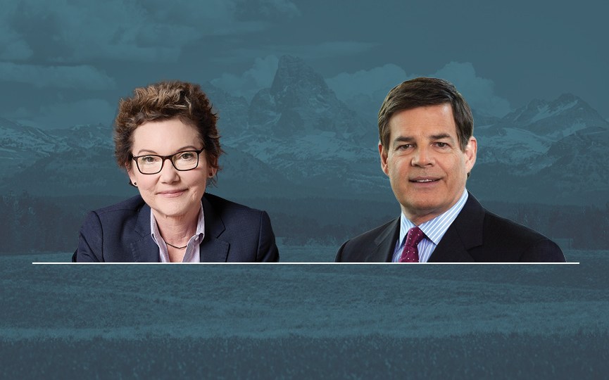
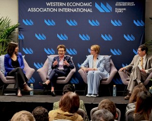
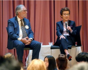
Rick Van der Ploeg, University of Oxford
Climate Policy and Asset Diversification

Date

Thursday, September 17, 2020

Time

SF 8:00am, NYC 11:00am, BERLIN 5:00pm

Location

Virtual

Rick van der Ploeg is Professor of Economics at the University of Oxford. He is Research Director of the Oxford Centre for the Analysis of Resource Rich Economies (OxCarre). He is also Research Fellow in International Macroeconomics at the CEPR, London, and Director of the Public Sector Economics programme at CESifo, Munich. His research interests are (international) macroeconomics and public finance with special focus on the economics of natural resources and climate change, political economy and development economics. He also has an interest in the economics of culture and higher education reform.

Download the paper (pdf, 804 kb)

Download the slides (pdf, 1.6 mb)

Seminar and Q&A recording (video, 55:48 minutes)

Transcript

Hide this section

Rick Van der Ploeg:

My call was at Christoph Humble and Holger Kraft, two finance guys from the University of Frankfurt. Christoph may be also available to answer questions. Before I go into that, I want to give a bit of an overview of what’s going on because not everybody may come in from the climate field. So on the A, I will discuss some stuff what’s been done so far or integrated assessment analysis of climate in the economy and then maybe also about risk and uncertainty. I’ll talk a bit about the motivation, giving some review of the empirics. And then C is the main part of my presentation, and I will finish with how we can do it better and some conclusions. So that’s the outline. A and B are fairly short, C is the main meat, and D is hopefully shorter as well. So most of the integrated assessment models. Out of the global economy often, and it typically have only one sector of the economy, one final good, and often they are deterministic. So the most famous one is the one which William Nordhaus got his Nobel Prize for it. That’s the DICE, the latest version is from 2016. He has a regional version of that. There are others like FUND by Anthoff and Tol, PAGE by Hope, and others. And all of these free are used a lot for policy analysis. Then there are lots of numerical energy models and they’re used to assess costs of meeting predefined emission targets. And then more recently starting with the paper by Golosov et al. in econometric, there’ve been a number of analytical integrated assessment models. So the Golosov et al. paper is effectively a Brock-Mirman model so that you can base, it’s essentially static because you can just write down the value function and you can get an analytical expression for the price of carbons. So about 700 people have cited that paper and have used it extended in all kinds of directions. Gerlagh and Liski have a paper which is also analytical and Lemoine and Rudik and American. If you have a paper, which is also more or less analytical. Now, almost all of these models, which I’ve mentioned on this through bullet, they suffer from a number of things, but one of them is that they’re suffered from too much temperature inertia. So that’s not true for Golosov et al., but for the others. So Simon Dietz in an earlier seminar already explained that that will lead to lower carbon prices and we explored those effects. Most of them don’t have stochastic. Sometimes they put stochastics in it, but they often use Monte Carlo simulation, which gives very misleading results. And Golosov et al. make the assumptions that elasticity of intertemporal substitution and the coefficient of relative risk aversion are both equal to one, they effectively have log revenue preferences. So that means that all effects of uncertainty drop out in the expressions for the price of carbon and that’s kind of not very useful for stochastics. But there has been a huge wave in papers in the last few years, allowing for stochastics also tipping points using stochastic versions of DICE. I thinking of Gollier, Crost and Traeger, Jasen and Traeger, Lemoine and Traeger, and particularly, a huge paper, which had a lot of work by Cai and Thomas Lontzek in the GP. And then there’s also some other papers would start to become kind of appeal to asset pricing. So the best known paper dispatchers, Daniel, Letterman and Wagner. So I’m just still getting this overview. So they do do the in continuous time, but their use of a binomial tree, but seven periods. So you can basically do the an Excel sheet if you want of an asset pricing mode. So that’s asset pricing 101, if you want. And then the main result is that they argue that the optimal carbon price declines over time. That needs two key ingredients. The first ingredient is that there is a preference for early resolution of uncertainty. So the Epstein-Zin preferences, that means that the risk aversion exceeds the inverse of elasticity of intertemporal substitution. And the second key ingredient is that they need a gradual resolution of damage ratio uncertainty. So if time goes along and there’s a shock to them, it just appeared, it can’t happen again and that means you don’t have to price for it in the precautionary way. So basically, it’s those two ingredients which lead to declining price parcels for year two. This paper by Olijslagers et al., they revisit this paper with continuous-time. So it kind of 201 asset pricing model and show that the optimal carbon price consists of a rising component proportional to GDP and a declining component that depends exactly like in the Daniel et al. paper that depends on uncertainty considerations. And the main point of it that extension is that the first component usually swamps the second component. Yeah, so basically, what I read for this, it’s not clear that the path will be declining because there is a component of the path because damages are proportional to GDP, the optimal carbon price will be proportional to GDP. So, but it will, it will nevertheless grow less than GDP because of this credit resolution of damage ratio uncertainty. In other work, which I did myself with de Zeeuw, you show that in a tipping model as a kind of a one-off temperature-dependent risk of a big increase in damages, then the carbon price will decline after the tip. But today, we won’t look at that type of stuff, today, I will look later on at recurring Barro-style disasters, where the incidence, which is Barro-style disasters are very carbon and macro and where the incidents of these climate-related disasters, some of these, are increasing with temperature. So they’re not one-off irreversible disasters, but they’re recurring disasters. And then the results are very, very different. Before I move on to do this, to set the story of that, I want to say something about a one sector story. So I have an old, well, it’s not a recent paper they’re from the Bremer, which is called the risk adjusted carbon price. So I just want to flag this in just two or three slides, where you basically can derive if you have one sector dynamic stochastic general equilibrium models, you may have correlated risks, you may have skewed distributions, you have mean reversion, and you may have convex damages. So the idea is there is still risk. That’s particularly important ’cause the effect of the carbon stock on temperature, so the effect of the amount of carbon in the atmosphere on temperature, it’s called the climate sensitivity, and that thing has a very long tail to the right. And what we show is that that tail type on uncertainty, normally like tipping points, is a huge driver of carbon prices. So skewed uncertainty is something which particularly drives up the carbon price. So I won’t bore you with how we do that. It’s using methods, which I have not seen in economics before, but they use perturbation methods in particular, perturbation methods and the method of multiple scales to allow for the fact that some parts of the model occur much more slowly than other parts of the model, and then maybe get some insight to do precaution, insurance, hedging motives. So just to give you an idea, all of these models, including the goal of Golosov model and not with carbon prices like this in the one sector version. So basically, what you see from there is there’s the carbon price, p, is proportional to GDP or aggregate consumption, some measure of aggregate economic activity. It usually grows global GDP. Theta is a coefficient which has to do with damages and then you divide by some discount rate. And the discount rate is very well familiar for a those in macro because it’s just a risk adjusted return rate of interest. In the absence of uncertainty, it just basically the Keynes-Ramsey rule, a little older. So if you look at a discount rate, it’s being used to discount all these damages. And if you forget for the time being all these delta terms, I’ll come to those in a second, you basically see that the price of carbon is the present is counter value of mass of damages, that’s the stuff on top, and then you divided by the social discount rate, the risk adjusted social discount rates, and that’s given by this expression here.
It’s, of course, if policymakers are more impatient, the big part of the debate was that stern said as 0.1% and notice it as 1 1/2%, so Debbie see that already. It depends on the growth rate G is to grow rate of the economy, if the growth rate is high, then future generations will be very rich. And then maybe you will want to have a higher discount rate and want the price carbon less because current generation, say, why should I do it if you will future generations they’re much richer. It depends on this gamma, which is the inverse elasticity of intertemporal substitution or it’s really a measure of intergenerational inequality aversion. Then there’s a minus G term and that’s just to allow for the fact that damages are proportion of GDP. So you must have a growth corrected rate of interest and that’s another term. Then the prudence term is familiar to all of you who do macro because it’s like a Kimball term, it’s like a prudential term. It has to do with the fact that the reveal of the utility function, deferred the revenue utility function has to be positive, is proportional to the volatility of the economy, which is Sigma k squared. That’s the volatility of the aggregate capital stock, is proportional to the question of risk aversion, theta, and is proportional to the cautions of relative prudence, which is one plus gamma. Then there is an extra term that’s the last time, not many. It’s very important to see that sometimes there’s a beta in front of that because it’s really the beta term, but the beta is one because damages are proportional to GDP. So it’s the idea that in the feature stage of nature, the damages are very strong, then the economy is very strong as well. I that mean you adjust your interest rate up and you need to price carbon less. You need to undertake less climate action because we have self-insurance anyway. And their final term is if there’s any decay of atmospheric carbon. So this kind of sums up a lot of levels going on. Now, you immediately see that if gamma and equal are equal to one like in Golosov, there is zero effect. These prudence terms and insurance term, they cancel out against each other. So there you see there’s no effective uncertainty on the risk adjusted rate of interest, and therefore, no effect of uncertainty on the optimal carbon price. So this kind of sums up a lot of that stuff. So then there are these extra terms, Delta key, Delta love, and delta ck. So let me just show these in words. So the first to note those terms and allow the fact that if there’s uncertainty about the climate sensitivity, that’s the effect by which the temperature increases if you double the atmosphere carbon stock. If that uncertainty about that parameter is higher, then that pushes up the carbon price only if the relative distribution is right skewed or of damages are more convex. So the effect of the carbon prices, particularly largely the climate sensitivity is more uncertain and the distribution is more skewed. It’s also if the climate sensitivity shocks are less temporary and the discount rate is smaller. Then the second key inside G get, the damage rate volatility. So that’s uncertainty about the damage ratio is that there’s a lot of uncertainty about what damages are from global warming. It only has an upward effect on the carbon price if the damaged shocks are skewed. If they’re not skewed, there is no effect. And then if they’re skewed, the upward effect is particularly strong if the shocks are more volatile and more persistent. So these are two effects. If you look this that’s that term, Delta key and Delta love, but these are the effects of climate sensitivity, temperature sensitivity, uncertainty, and damage ratio uncertainty. Then I will do this for term delta ck and that’s a kind of a novel term, that’s a hedging term. And that hedging term is the effect that there are two effects. There’s a paper by Derek Lamont. I think it’s come out in the Gerry or something like that. And that he shows that if risk aversion exceeds one, in which we will assume here, then the hedging effect dominates offsetting effect. So he calls it slightly different, but basically that’s the effect. So let me give you the interpretation before I delve into our paper. So the interpretation is as follows, suppose in future states of nature, asset returns are negatively associated with temperature. Well, then if want the temperature beta is negative, and then it pays to invest more in fighting global warning and to push up the open price of carbon. So think of this. If you have industry selling winter garments, like big wooly jumpers or heating systems, then if it’s getting hotter, then they’ll put out of business because nobody wants these big wooly jumpers anymore. So, and that’s the reason why that pushes up the social cost of carbon, pushes up climate a price to avoid is global warming. But of course, if you had a sectoral model, there maybe industries producing Champaign in Sussex or wine in Sussex and in the South of the United Kingdom. Now the champaign there is at least as good in quality as in France, just because of climate change, then the beta is positive. And you could imagine those wine producers, they will run down to have a lower cost of carbon and that come out at formula. So they want to price carbon less vigorously because a bit of global warming puts these farmers in South Sussex into business. And then another way of looking at this is kind of the correlation between temperature sensitivity uncertainty, and between asset returns. But there’s also a correlation between asset returns and the demonstration. Suppose that in future states of nature, asset returns are negatively associated with damage ratio, then the damage beta as we call it is negative and it must push up the cost of carbon. The idea is that they have in the future state of nature there’s a lot of damages, then probably the stock markets go down and that sense of damage ratio is negative and the costs of carbon is pushed up. Now, half of me is Dutch or half of me is from the Netherlands. And there’ll be might argue it’s the other way around. We have a huge industry which makes money out of climate change because whenever there are floods or whatever, all these Dutch shipping companies come in, salvage companies come in, water defense companies too comes in. So you can argue that for a large part of the Dutch industry, their asset returns benefit if there is a big damage ratio. So then for those type of costs, they would want the lower cost of carbon. So if you want this term here captures these row k key and row K lambda are there are these correlation coefficients between these two types of uncertainty, between the uncertainty in the economy, k, and the uncertainty in the climate sensitivity key, or the correlation between the economy and lambda, which is the damage ratio. So this is as far as I can get with asset pricing, looking at the Daniel et al. paper in the “Proceedings of National Economy in Sciences” and this is the paper if I’m the dream. And there a few other papers around. There still other papers also by Bonsel and others, we’ll go up to that top stuff. But today to follow a line, maybe go and look at two-sectors. So this is the main part of the paper. There are a few papers out there doing that, but this is what I want to do. So basically what should we do? So in a deterministic world, you might, if you want to have a green position, you want to immediately switch capital to the green sector in one go, boom, like that. But typically there are investment adjustment costs, maybe relocation costs, reallocation costs. So then full specialization takes time. But then in a stochastic world, other considerations come into play. We have a two-sector world, so just for simplicity, brown sector and the green sector, carbon-intensive sector, and a carbon-free sector. You might want to keep open the brown production sector as a hedge, also you might want to keep it open for some time because if it’s making a lot of money, it helps to finance the green tradition. So I’m going to eventually, I will come back to this, I’m going to look at free types
of negative effects of global warming on the economy. The first one is that global warming may negatively affect production just like in all these integrative rated assessment books, like in Nordhaus, but I’m also going to allow the second for a negative effect on depreciation rate of capital. There are papers by Melissa Dahl and others, who show up empirically a negative effect of global warming on the growth rate of the capital. So this is very similar to that and free, which is the more novel bit is every going to allow for risk of macro disasters. So that’s like Barro et al., but we make some of these macro as are climate-related. And then the incidents of the disasters occurring will increase with temperature. So there is not just one, but there may be three reasons to price carbon. So eventually what I want to throw at the end of it, I want to look at the effects of these types of damages and a wide range of uncertainties from the risk-adjusted carbon prices like what I did before, but also on the share prices and risk premiums are carbon-free and carbon-intensive types of industries. Now, before I do that, I think it will be helpful to one, there is a paper out there by Karydas and Xepapadeas. They do something similar. We have two endogenously Lucas trees, we have one exogenous Lucas tree, which can be painted green. But it’s a related paper, I won’t say much more about it, but it’s very useful to read it as well. So I’m going to, before I go to these effects to show these effects in the model, I think it’s useful to briefly look at some of the empirical literature. So the empirical evidence is mixed. There are two great papers, particularly the Bolton and Kacperzyk the first one, which is for the United States, they showed that carbon-intensive firms, think like steel cement, all majors, whatever, in the United States show higher stock market returns after controlling for size book to market, momentum, et cetera. And the idea is that investors already demand compensation for the carbon risk and they argue that this carbon risk premium cannot be explained via unexpected profitability or other risk premia. So they’re saying that the dirty assets get a higher rate of return because the investors otherwise wouldn’t buy them, they need a higher rate of return to compensate them for the risk that they may go belly up if the economy certainly transitions more quickly than is now expected towards a carbon-free state, And the second Bolton and Kacperzyk sheet paper does the same for a cross section of 14,000 firms in about 80 countries. And then they show evidence also for this risk premium, carbon-risk premium, and that it rises for carbon-intensive stocks. And these studies also indicate that institutional investors are already divesting away from the carbon intensive firms. But however, there were other studies, for example, there’s a recent paper by In, Park and Mong, and they look at 736 US firms and they look at an EMI portfolio, basically carbon-efficient minus carbon-inefficient. And then they show that generates huge abnormal returns. So an investment strategy of going long on carbon-efficient firms and going short on carbon-inefficient firms would earn abnormal returns between 3.5 and 5.4% per year. And that’s not driven by the low interest rates after the global financial crisis, it just tends to be out and also they also find that carbon-efficient firms are good in terms of financial characteristics and governance. So there’s that. So that’s another empirical study. So there’s another paper by Garvey, Iyer, and Nash, and they showed that firms would have a lower ratio of carbon emissions to sales should be one, the E in the ESG, are less dependent on carbon, has stronger future probability, and higher stock returns. Well, that’s kinda the opposite of what Bolton and Kacperzyk found. So it’s mixed empirical evidence. There’s another paper by Plantinga and Scholtens and they look at 7000 companies and they find that investment portfolio that exclude fossil fuel production companies don’t perform worse than unrestricted portfolios. So they suggested that if you divest from fossil fuel companies, it doesn’t have performance at all. So I’m just putting some papers out there, that people are trying to begin to use, finance guys are trying to find out the effects of climate change on that. A paper I quite liked was this paper. It’s just being presented at the Seabra seminars. It’s by Donadelli, Gruning, and Hitzemann, and they just focus at the fossil fuel industry. A good thing about it is you don’t have to worry about classification issue. So they have better econometrics and they’re interested in changing the value along trends in climate change environments. So they get these awareness of climate change risk from Google search and they find it’s closely coordinated environmental policy strategy. So they do some machine learning and do some linguistic algorithm to get those data. And then they explain the market to book ratio of about 4000 firms over the period of 1970 to 2018. And then the panel regression to control for a market-wide valuation, a lot of other trends in the control for cash to assets, debt to assets, log assets of x assets, and R&D sales. So what they then find is that there is not only that stock market value of US oil and fossil fuel firms from a lot of the last 20 years compared to other firms and during Corona crisis, they fall even more. But markets have started to price in the climate transition. So they find a strong least significant and quantitatively important negative coefficient on climate awareness index. So what they’re finding is that this risk premium, if you will, these found by Bolton and Kacperzyk are there, but they are growing and they are related to this climate awareness as picked up from Google searches and other data. So I find that interesting. They also have a model which is a bit related to ours, but it’s nevertheless it’s different analysis, continuous-time, well, anyway, you might want to look at it. So then there is some related literature, a number of papers in particularly the paper by Barnett, which I’m a big fan of, I think it’s an absolutely wonderful paper. We had an earlier paper vd Ploeg and Rezai from vd Ploeg and Rezai maybe show the effects of the risk of policy tipping on the market valuation of oil companies. So the idea is that in the market, people don’t really know whether the, I mean, Obama before, that’s great, things are green, the government is going to do climate policy, and then suddenly Trump came along. That was a stochastic shock because nobody was aware that Trump was going to win. So there’s always policy uncertainty because of the risk of policy tipping. And we then find out that that policy uncertainty and costly adjustment of capital stocks can lead to stranded assets. And you can also adopt the game-theoretic approach, it kind of a race to burn the last form of carbon. If you know there’s going to be a cap, you’re only allowed to be burning so much more carbon, and then it’s done, then you can imagine that all these firms and trying to get it out of the ground as quick as possible before it becomes worthless, before they really get hit by the risk of stranded assets. But then there’s this nice paper by Barnett, which models, it’s a bit like our paper, but it’s very nicely done. It’s an uncertain arrival time of policy change generates, again, a run on oil, it’s like a race to burn loss. It’s a run on oil. So you get falls in the spot price of oil and the market valuation of companies, you get an increase in green energy prices and higher temperature. So in this paper, he will also calculate a stochastic discount factor as we do, they look at asset pricing implications, and then they, again, also find evidence for potential carbon bubbles. So this whole idea of risk of stranded assets, the idea of there being a potential carbon bubble is a type of research area that’s not getting quite hot. It is not that many papers out on that, but that’s an important area. I’d have a little bit to say on it, but not that much. So sort of just what I wanted to say
. So now I come to the main meat of our stuff, which is our approach is the paper Humble and Kraft. So to avoid carbon emission and global warming, emissions-free technologies and renewable energies must substitute for fossil fuel. So a lot of people vary on how urgent it is to transition to become a free economy. Our interest is in interplay between financial considerations and policies to mitigate climate change. So the key questions are, does financial need to diversify hamper or help the fight against climate change? And the second, how does climate change affect pricing of green and dirty assets? So we’re going to be interested in the subtle dynamic interdependence between the financial goal to diversify assets in portfolios and the environmental goal to cut emissions. So we therefore put forward two-sector continuous-time DSGE model of economy in the climate, two capital stocks, to energy sources, the green-sector has carbon-free energy as input, the dirty sector requires fossil fuel, whose combustion is lead to emissions. You can reallocate capital from dirty to the green sector, but that’s costly. And you can do invest of course, but that’s also subject into that from adjustment costs. The growth and capital needs sector is subject to Barro-style, disaster shocks, it’s also subject to climate related disasters shocks and to normal macro shocks, like premium motions, if you want. We’re going to have Duffie-Epstein preferences. So we separate risk aversion in the temporal substitution. So we can calibrate to get a release disaster shocks, a high equity premium, and a low risk-free rate in the data. We usually thing that Simon Deitz also talked about that we have temperatures linear function of cumulative emissions. So emissions are proportionate to fossil fuel use and temperature negatively affects the TSP, the depreciation rate, and the risks of climate-related disaster. So that’s, in words, our model. So at the preview of our results, you diversify until there is a balance between green and dirty capital in our calibration, that means 50/50, but the environmental perspective issue, you run down the dirty capital stock completely. So the latter doesn’t occur with DICE damages, which are only modest, but does occur if the damages from climate change are much more severe or the different damages are taken together, then you will run down the dirty capital stock together. But in general, there’s a trade-off between diversification and climate change policy. So diversification considerations may in a plain vanilla, Nordhaus model, will prevent driving the dirty capital talk to zero. So we will analyze the dynamics of the risk-free rate and the risk premium during the green transition. So the risk-free rate will fall. The rising temperature is a preview of the result and the risk premium are only significantly effected if the risk of disasters increases with temperature. L is the impact on risk premia is moderate. So for example, if you’re just looking at the Nordhaus damages, there’s no big effect on risk premium. So the big effect and risk premium comes for this temperature-dependent risk of disasters. Okay. So this is my introduction and now I come to slightly boring part of the talk, where I will go for the model. So the model is an AK growth model, AK macroeconomic growth, but it has two-sectors. It’s very simple and in some ways it’s too simple and we did it deliberately. It’s barely an illustrative model. So for example, we have perfect substitution in consumption where we may want to have imperfect substitution in consumption. We have two sectors, sector one is the green sector and sector two is the dirty sector. F1 is renewable energy and F2 oil and gas and coal. And you see that lambda T and these two-sectors are negative effects of temperature on TFP. It depends on capital K, F for fossil fuel, and then you see K, L, that’s the typical AK formulation that the productivity of labor depends on the aggregate Y to capital stock. So you can ride the first equation as the second an equation. Then, then B how allow for intertemporal and intersectoral investment adjustment costs. We allow for temperature-dependent depreciation rates and independent geometric Brownian motions with correlations between the capital stocks. So for the disaster risks, we have a constant jump intensity just like in Barro, but temperature-dependent jump intensity, a bit like Karydas and Xepapadeas. So that leads to these equations. The exact mathematics is not so important, but you get an equation for the growth of the capital stock in the green sector, K1, and an equation to grow from the capital stock in a brown sector, K2. You see the investment, I1, and then you get a minus 1/2, I1, I1 squared over K. That’s a standard , Iyer style investment adjustment costs. Then R is plus R in the first equation, minus R on the same equation, that mean you relocate capital from the dirty sector K2, to the green sector K1 and there may be some adjustment costs associated with that. Then you see that the depreciation rates are delta 1 K plus term theta 1 T, which is temperature. So you see the depreciate raise of capital or an increase in functional temperature. And that’s the second XML in the model. And the term K1 sigma dW1, that’s just a geometric Brownian motion, if you want, that’s just the normal macroeconomic uncertainty. And the last term on the second line of these models are the two Fosun-style disaster shocks. The LE it amounts indicated by a subscript e are the Barro-style, and the ones indicated by c are the climate-related disaster shocks, which we assume to be the only differences that we calibrate in a way that the intensity of those occurring increases with temperature. So that’s the third reason for why you have a reason to fight global warming. I already said that the model of temperature is that easy. It’s now a fairly standard practice in the IPCC. It goes back to original paves by Matthews and Allen. And basically, it’s not bad at all to assume that temperature is just linear function of cumulative emissions. We, again assume some noise there and be calibrate that and that model of temperature. Then following Cochrane et al., that’s a key paper for us in finance, they said equilibrium dividends equal to aggregate consumption, i.e. if you have an unleveraged claim on aggregate consumption, So C is the sum of the two difference of the sectors. So a critical remark here is that I would have preferred, and we will do that in a next generation of the model, I suppose, they have a leverage claim on aggregate consumption because then you can distinguish between the volatility of consumption, which is, and the volatility of capital GDP because these are very different and you have an extra parameter by which you can, the difference between the volatility of consumption and the volatility of the asset returns, the growth rate of consumption, the volatility do that, and the volatility of asset returns are the same as these AK models. As we know that the volatility of asset returns is much higher than the volatility of real economic activity. So to allow for that, you really need to have a leverage claim on aggregate consumption. We have not done that here, but that’s something on our agenda of work to do. So, and then on the bottom, you see the Duffie-Epstein utility function. All you need to know is that we’ve assumed without loss of generalativity that elasticity of intertemporal substitution equals one or the risk aversion is gamma and can be much larger than one and typically, it will be much larger than one. So again, do not look at this equation. So all that whole model can be summarized by this ugly Hamilton-Jacobi-Bellman equation, where we have a large number of state variables. We have K1, K2, and temperature. So if the two capital stocks on temperature, we do trick, which is useful for those people who like to solve these things with finite differences, is to reduce the state space. So we can use a, I’ll show that in a second. But before we do that, we will show you the optimality conditions. The optimality conditions give investment as alway
s. The investment ratio is I over K respond to the Tobin’s Qs positively. So higher Tobin Q means higher investment rates. The Tobin’s Qs are related to the marginal value of capital divided by the marginal value of consumption. The optimal reallocation of capital if the Tobin Q the clean sector is higher that the Tobin’s Q in the dirty sector, then you relocate capital from the dirty sector to the green sector, then our R is positive. And then these two equations there are just a mass of productivity conditions for fossil fuel and for green energy. So the left hand one is for green energy, it’s just a cost of green energy what we want and the mass of product fossil fuel is equal to the cost of fossil fuel, B2, plus something related to the Pigouvian tax from using one unit of fossil fuel, which has given on that bottom expression there. So this is the theorem we use to make the model easier to solve. So we define a share of dirty capital. This is a share of the capital in the Brown sector divided by the total capital stock. Then you can just basically this fair insurance that you can just solve the reduced-form Hamilton-Jacobi-Bellman equation in terms of S and T, just intentional share of dirty capital on temperature, rather than terms of those three variables. And we can actually write down the value function exactly as it’s given there in expression 3.9 is proportional to K to the one minus gamma and a reduced-form value function just depends on T and S. This makes it computationally so, so much easier to solve, and otherwise, it would have been a actually numerically, a bit of a nightmare.

Glenn Rudebusch:

Rick, we have about 20 minutes left in the presentation.

Rick:

Okay, I’m fine

Glenn:

Great.

Rick:

So then we got the optimal social costs of carbon, which he gives them expressions there. And let’s then go to some numerical results. So you may want to look at this for not too long, I’m not going to discuss the whole calibration, but you might read from that that risk aversion is 5.3, which is bigger than one. Yeah, it’s calibrated, the world economy was down about $76 trillion. We have an initial share capital is 94%, is much too high. And we have green productivity. So we match a lot of that model. I will say a little bit about later. So now you see here, the whole model. A crucial one is that TCRE that shows that for every trillion tons of carbon, the temperature goes up by 1.8 degrees Celsius. So show you a little bit more, the model is calibrated to do business as usual. Some key things, share of energy is 6.6%. We matched the adjustment costs to match the risk-free rate of 0.8% and average equity premium of 6.3% and a Tobin’s Q of 1.5. And that gives us this risk aversion of 5.3. So we matched the volatility of consumption, divided by our portfolio and Wachter paper. So we get sigma on sigma two equal to 0.02, and we choose the reallocation parameters, the reallocation of capital across two-sectors, such that global warming is about four degrees after 200 years. So that’s in line with Nordhaus’s model. And the 1.8 degrees for the transient climate response to cumulative emissions come directly from these papers by Allen and Matthews. And we calibrate emissions intensity, that’s a function of time. So it’s a business as usual emissions in the DICE model actually. So what we do is we matched with the real data, but for some stuff, which we don’t have good data, we match it to what we know from DICE so that you can compare with DICE. So they give you some example. Here you see that basically all these stocks are on top of each other, it’s our model and the DICE model. So we capture exactly the emissions in the DICE model and the business as usual, we capture temperature on the business as usual, and we captured emissions intensity per unit of fossil fuel. So that’s why we that’s what we’ve done. So there are three types of climate externalities, three types of reasons to price carbon. The first one is this Nordhaus damages and basically it’s quadratic in temperature. So the damages to aggregate production is that familiar expression from Nordhaus. The second one are ones the damages to the disaster shocks, calibrate the disaster shocks, and they should at the incidence rate. So lambda c is the incidence rate increase in temperature so that the higher the temperature, the higher the instance rate, and if you want, the smaller the interval between disasters. And then the last term is the effect on the depreciation rate of temperature. So that’s a Melissa Dahl effect. So we follow Barro and Jim for the normal disaster shock. So we have an average consumption loss of 20% if the disaster occurs. So an annual disaster risk of 3.8% allows us to calibrate the model and then they basically use a power distribution. For the climate-related disasters, it’s a bit more important. It’s not that different from Karydas and Xepapadeas. They use that data for 42 countries over a period of 1911 to 2015. And then we ended up if a disaster risk intensity of increasing in temperature, 0.096 time temperature. The mean jump size of climate disasters is about 1.5%. Hence, that’s the size. We again, use a power distribution for the recovery rate, where the size of disaster shock indeed as a mean value of 1.5%. So let’s show some effects. So this is where it becomes important. So here we see three columns. So the first columns are when the model only looks at global warming damages to GDP, so Nordhaus damages. The second column is when there are only a damages due to the fact that there is a bigger intensity of climate disasters. And the third column is there only the effect of temperature on depreciation rate. Now, what you see is that the dotted lines are hypothetical scenario without damage on climate change. what do you want to see is that black lines, the dark black lines, show a declining share of dirty capital. Notice that they don’t go to zero, they go to somewhere like 0.3. If there were no climate damages, so that’s the, the, the doc dotted line, then they go following the, the Cochrane theorem, the Cochrane paper, 2009 paper, they go exactly to 50%. So the idea is if you don’t take care of the climate changes considerations, then the share of dirty capital go to a balanced capital stock of it’s 50/50, the way we’ve calibrated the model, and then it goes to 50%. The black line is below the dotted line in all three columns. And that’s to reflect the fact that you actually want to use less of dirty capital because of the climate. Now, if you look at the gray lines, the dark gray lines and the light gray lines, then these correspond to when the damage parameters are twice as high or three times as high. So what you then see is if you make them just more important, the black line shifts done. So then you give less consideration to diversification objectives and you give more weight to fighting climate change. So you bring down the share of dirty capital much more. And I expect in the second and third column, you bring for the light gray lines, you bring the share of dirty capital in 2100 down to zero altogether and as a result, temperature is much, much lower than it is on the business as usual or on of the black line. So I think the main insight for here is that the dirty capital share is brought down to more than you would do for pure diversification is because of climate change. It doesn’t necessarily bring it down to zero unless damages are very strong and that’s particularly, it’s not so much the case for the Nordhaus damages, but it’s true that if you have a temperature-dependent incidents of disasters or if you have these Melissa Dahl type of effects, where temperature increases the depreciation rate of capital. So that’s our intuition and I think if you put all the damages together, all the free columns together, you will definitely go to drive to under share of dirty capital and to find that time to zero. So this is the next thing, and this tells us a little bit about hedging. So again, we have a free columns. So the three columns are, the left column is, again, for the Nordhaus damage. The middle column is for disaster rate damages, so the incidents of disasters are temperature-dependent. And the third column is when the depreciation rate is the temperature-dependent. Now, what do we want to pick up from that? So what you want to show is that the black lines, so the dark black lines, if you want, are the results for the benchmark case, where the correlation between the Brownian shocks affecting the green and dirty sector are zero. And then the gray lines show the results when there’s a positive correlation of a 1/2 and the light line shows the effect and there’s a negative correlation of minus 0.5. So what you then see is that if the two shocks are positively correlated, if they’re negative recorded, let me put it that way, then there’s a hedging of comes in. So the light line, therefore, and that’s the reason why the light line, the share of dirty capital first goes lower than the black line and then goes higher. That’s in the case of positive correlation, the dark gray line is higher than the dark black line and then goes down below. So maybe to kind of ride down to intuition here on the sheet if the Brownian motion shocks are negatively correlated, the light gray ones, the diversification motive is amplified. So you get a quicker transition to full diversification and the corporatization of the economy in the first stages, but after a while it reverses, and the opposite is true, and the economy keeps a high share of the dirty capital, the benefits from that to diversification. So there’s less climate action. Whereas we have positive correlation, that’s the dark gray line, the diversification model is weaker. So in the short run, the transition to the green economy slow down, but in the long run is speeded up and the economy
ends up being the lower share of dirty capital. Now, I would like to point out that both capital shocks are not only hit by these Brownian motion shocks, they’re also hit by disaster shocks, which the way these are models are carbon disaster shocks. So we are still trying to do that rum where we allow for do I think correlation correlations between the disaster shocks, but that’s not what these figures show. So I think this figure, the one that I’ve just explained, shows the effects of hedging that hedging really, that the correlation coefficients between the different types of shocks in the two sectors really matter for how fast and how quickly or how late you put your climate policy and how to trade-off has effective intertemporal, with diversification markers. So a few more minutes and I want to discuss the asset pricing implications. Well, we know from finance that the time zero price of a cashflow has given up there. The stochastic discount factor H is for Duffie-Epstein preferences given in the second equation and if Ito’s lemma that gives us an equation for the stochastic discount factors. These allows us to give the following results. It’s a bit daunting. So don’t propose to go through it, but equation 6.3 is the important one. And those who have done macrofinance, who would know finance will recognize this, but basically, the risk-free rate is basically a delta, which is the discount rate and you see is the affluence term minus gamma times that norm squared is the kind of the prudence term and if you have a disaster risk term that’s familiar as something similar you see in the Barro and Jim papers. And the last term is new as temperature to fruition. So the novelty of this proposition compared with earlier papers is that all these terms are endogenous and all of these terms are, you see, they’re norms. So they collect the effects of the different types of uncertainties on this risk-free adjusted to the risk-free rate. So, and then, and they also give expression for the market price of deficient risk and the market price jump risk on the bottom. So if you have time, I won’t go in a lot of detail for it, but let’s see a bit what’s going on here is that this stuff that extends Barro, it extends Wachter, Pindyck and Wang, and Karydas and Xepapadeas. So let see what it means. So if you look in our exercise, we just took it for one year. You can do it for any other years, it’s more or similar. This is what the decomposition pans out. So the state-dependent terms in decomposition of the risk-free rate, I just discussed in that propositions. So what you find is that you find the contribution of the disasters and contribution of the decomposition of that risk-free rate in this particular time. So the drivers are expected consumption growth, so that decreases in temperature due to damages, the decrease in the share of dirty capital as the optimal fossil fuel use, and as output, declines in the share of dirty capital. And two, the economy, it relocates capital at a higher rate and adjustment costs depress growth. So, as that happens, you decrease the share of dirty capital. The risk-free rate is also has a term for the negative precursory savings term. That temperature has a tiny effect, but the share of dirty capital has a big non-monotonic effect on this term. We explained it in detail why that effect is non-monotonic, and it has to do with these Cochrane considerations. And then we find that the temperature diffusion risk term is almost negligible. So you can see that here that this slide summarizes this table ’cause you see that these risk-free rates depend on temperature, they depend on this share of dirty capital, and then basically this slide gives you the results. So we can price the trees. So we can do for any stream of future evidence, we can get asset prices, and we can actually also, that’s also how we calculate the cost of carbon incidentally. So here you see some effects, and I’m wonder what it is, and I’m almost there. So here you see the Qs, the risk-free rate and equity premium. So what you find is that the dark lines show you the effects when the share of dirty capital is 95%, the gray lines share of dirty capital is 50%, and the light gray lines when they’re point of 0.05%. So they plot the Tobin’s Q of the green assets and, B, to show the Tobin’s Q to dirty capital stock. So let me, again, it’s probably easier to explain it here on the slide. Well, that figure shows you the Tobin’s Q for both the green and the dirty sector decline in temperature. So if you see that they both decline in temperature. The book to market ratio increases in temperature. So if we’re giving capital, marketability decreases the temperature for both assets. The Tobin’s Q of the green aasset increases in the share of dirty capital, hence for a given capital, green asset has a higher market value if the economy is more carbon-intensive. The opposite is true for the carbon-intensive assets. So the behavior of the risk-free asset is, as we already discussed, the green and brown equity premiums depend positively on the clean and dirty share of capital and they are hardly affected by temperature. So what do you find is that if carbon is correctly priced, the green premium is higher than the brown premium, but ethically of course, you’re optimally adjusting climate policy. Bolton and Kacperzyk find empirical results for what arguably is the, if you want, the business as usual situation, and then they do find also a carbon-risk premium as data. So the drivers of these risk premiums in 2100 are, again, the risk premium on the green asset increases in temperature and especially in your share of dirty capital. Also true for the expected ex-divdend green stock return, which increases sharply in the share of dirty capital. So if the share of dirty capital is high, the green stock pays fewer dividends, but after green transition, the green asset pays higher dividends. So in the beginning to share a dirty capital is still high and then the green stock doesn’t pay so much dividends, but once the green transition has taken place, the green asset pays high dividends. So there’s a positive correlation with share of dirty capital and the greens Tobin’s Q. So I end this time series solutions just and then we see also five and 95% confidence bounds, and we show business usual. So here you see the familiar results. It doesn’t look that different from a one sector model. If you look at output and again for the three types of externalities, it’s lowered as the dotted lines, we see that for the consumption rate, it’s initially higher and then later it’s lower than business as usual, we see emissions being really curved quite a bit in all three cases and that’s a jolly good thing. And then if you look here at the share of dirty capital, again, with the five and 95% confidence bounds. We see in all three cases, they come down quite a bit. Temperature is also brought down quite a bit compared to the business as usual and they hit on the bottom, you see the expressions for the carbon tax and also the confidence bounds for the carbon tax in each of the three cases. Basically, you see that their costs grow as the economy grows. If we kill productivity growth in the economy, then the carbon taxes will be much flatter. And these are the type of results which may hide some of the stuff going on with the diversification and share of dirty assets, but they are very similar to what you see on risk stochastic one sector models. So some results are that the share of dirty capital in the hypothetical case of zero climate damage goes to 50% as I said before. But when the government prices carbon to fight global warming, the share of dirty capital goes down further with 25 to 30%. Crucially, it doesn’t go down to zero and we’re emphasizing that as some positive amount of dirty capital is kept for diversification purposes. And then that, of course, hampers to fight against global warming. So here see, again, the effects on asset pricing quantities. So what you want to see is that the risk-free rates, if you look at that, what you should see is that the dotted lines are much lower than t
he dark lines. So I show you why that is and you’ll also want to look at the middle column and there you see, there’s much more action in the risk premium that in the first and the third column. So this is literally the last slide. So the risk-free rate falls much more strongly over time if carbon isn’t price like in business as usual. And the reason is when you think about it is that there is, if it’s not priced, then the market engaged in the precautionary savings to cope with the inevitably growing climate damages that will result on the business as usual. So if you’re pricing carbon optimally, the risk-free rate doesn’t have to price. It doesn’t have to follow up time so much because we don’t have these large growing climate damages. So only for the disaster impact, that’s the middle column, do we see it’s made significant gradual rise in both the green and the dirty risk premium as the temperature rises. So the dirty risk premium depends on the dirty capital share and temperature in a nonlinear way. So you get the snake-shaped evolution of the dirty risk premium over time for the level and growth damages. So it is mainly disaster damages to do the work. So the risk premium is really affected by disaster damages. The risk premium is higher and increasing and it’s triggered by additional Poisson shocks, collaborative Poisson shocks, giving rise to an extra component in the risk premium that last component in proposition 6.1. So since the jump intensity of these shocks rises with temperature, this extra component becomes especially important business as usual and asset holders demand to be compensated for these increasing climate risks. And that kind of explains the empirical results of Bolton and Kacperzyk. So I think this is what we have. So I leave it at this and open the floor for questions.

This seminar is part of the Virtual Seminar on Climate Economics series hosted by the Federal Reserve Bank of San Francisco and is open to everyone interested in research on the economics of climate change.