The December 12, 2006, statement of the Federal Open Market Committee (FOMC) said, “Readings on core inflation have been elevated, and the high level of resource utilization has the potential to sustain inflation pressures.” The link between “inflation pressures” and the “level of resource utilization” is formalized by the Phillips curve, which says that short-term movements in inflation and unemployment (a measure of labor resource utilization) tend to go in opposite directions.
- Methods of forecasting inflation
- Quantitative forecast comparison
- Policy implications
- Conclusion
- References
The December 12, 2006, statement of the Federal Open Market Committee (FOMC) said, “Readings on core inflation have been elevated, and the high level of resource utilization has the potential to sustain inflation pressures.” The link between “inflation pressures” and the “level of resource utilization” is formalized by the Phillips curve, which says that short-term movements in inflation and unemployment (a measure of labor resource utilization) tend to go in opposite directions. For example, when strong economic activity makes the labor market tight, inflation is likely to increase. Technically, “tightness” in the labor market means that the unemployment rate is below its natural (or equilibrium) rate, a measure that is not directly observable but is derived from estimates. Pioneering research by economists Edmund Phelps and Milton Friedman during the 1960s asserted that monetary policy could not keep the unemployment rate permanently below the natural rate–a view that is now universally accepted. Phelps is the most recent recipient of the Nobel Memorial Prize in economic science. Friedman was awarded the same prize in 1976.
A much debated question among economists is the usefulness of the Phillips curve as a tool for forecasting inflation (see Lansing 2002 for an introduction to this debate). This Economic Letter presents some quantitative comparisons between a Phillips curve-based inflation forecast and an alternative forecast that is constructed as a weighted moving average of past observed rates of inflation.
Methods of forecasting inflation
The Phillips curve is a commonly used framework for forecasting inflation, but difficulties in knowing the true value of the natural rate, together with empirical instabilities in the inflation-unemployment relationship can lead to significant forecast errors. A simple estimated version of a Phillips curve can be obtained by regressing the one-quarter change in (annualized) quarterly inflation on the lagged unemployment rate and a constant term. Inflation is measured using the “core” personal consumption expenditures (PCE) price index, which excludes food and energy components. The estimated coefficient on the unemployment rate is the “slope” of the Phillips curve. The ratio of the estimated constant term to the absolute value of the slope coefficient is an estimate of the natural rate of unemployment.
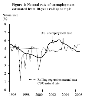
 Figure 1 plots the natural rate estimates obtained from a series of 10-year rolling regressions. The estimated value of the natural rate is quite volatile for sample periods that span the late 1990s. Since 2001, however, the rolling-regression estimates are more stable and track reasonably well with the natural rate series constructed by the Congressional Budget Office (CBO). Although not shown, the rolling-regression estimates of the slope coefficient also exhibit a fair amount of variability–reflecting the fundamental imprecision of the link between inflation and economic activity. The magnitude of the estimated slope coefficient has approached zero in recent decades, suggesting that the Phillips curve has become less useful for forecasting inflation. Along these lines, Federal Reserve Bank of Richmond President Jeffrey Lacker (USA Today 2006, p. B8) recently stated his view that “Moderating growth doesn’t change inflation. Central banks change inflation.”
Numerous research studies have demonstrated that forecasts of U.S. inflation based on empirical Phillips curve models can frequently underperform simple alternative forecasts that only employ data on inflation itself. A naive random walk forecast says that future inflation will be the same as current inflation. A study by Atkeson and Ohanian (2001) showed that a random walk forecast outperforms a Phillips curve-based inflation forecast from 1984 onwards.
A random walk forecast uses data only on the most recent inflation rate. A more general forecasting approach uses a moving average of past rates of inflation, with recent data receiving more weight than older data. This “weighted moving average” forecast is known to be more accurate when inflation movements are governed by both temporary and permanent shocks. The underlying assumption is that temporary shocks push inflation away from a long-run target rate but permanent shocks can shift the target over time.
The optimal weights assigned to past inflation in the forecast rule are governed by a mathematical formula that depends on the ratio of volatilities of permanent to temporary shocks. A higher volatility ratio means that a larger fraction of observed movements in inflation are viewed as permanent, thus increasing the weight assigned to recent data in the forecast rule. The volatility ratio can be identified from the data by measuring the persistence of one-quarter changes in the inflation rate, as shown by Lansing (2006). The methodology reveals a downward trending volatility ratio over the last decade, indicating a reduced likelihood of a permanent shift (either upwards or downwards) in the Fed’s inflation target. This evidence is consistent with the idea of “well-anchored inflation expectations” in describing the current environment (see, for example, Williams 2006).
Quantitative forecast comparison
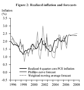
 Figure 2 plots one-year-ahead inflation forecasts together with realized inflation data over the period 1996:Q1 to 2006:Q3. The distance between the forecasts and the realized data represents the forecast error. The metric for assessing forecast accuracy is the mean squared error of the forecast.
Each quarter, the latest Phillips curve regression equation is iterated four quarters ahead to compute a predicted average inflation rate for the coming year. The predicted trajectory of the unemployment rate is constructed by assuming that the prevailing unemployment rate will gradually adjust to the most recent estimate of the natural rate.
The weighted moving average forecast is constructed using the weights implied by the volatility ratio identified from a 10-year rolling sample. Forecasts beyond one quarter are set equal to the one-quarter-ahead prediction, reflecting the idea that the best forecast of the future inflation target is the current estimate of the inflation target.
The weighted moving average forecast outperforms both the Phillips curve and a random walk forecast over the full data sample that runs from 1975:Q1 to 2006:Q3. The weighted moving average also delivers the best performance in two out of three subperiods, namely, during the volatile inflation era from 1975:Q1 to 1984:Q4 and the stable inflation era from 1996:Q1 to 2006:Q3. The random walk forecast (not shown) does slightly better than the weighted moving average during the intermediate period that runs from 1985:Q1 to 1995:Q4. These results are in line with previous studies which find that simple inflation-based forecast rules can routinely outperform Phillips curve-based forecasts.
In Figure 2, the Phillips curve predicts a mild upward drift in core PCE inflation over the next two years as the unemployment rate rises towards the natural rate. The weighted moving average predicts a slight decrease in core PCE inflation from 2006:Q3 to 2006:Q4, followed by a leveling out thereafter at the current estimate of the long-run inflation target (which is slightly below 2.4%).
The unemployment “gap” is the percentage-point difference between the natural rate and the prevailing unemployment rate. In addition to appearing in Phillips curve models, the gap plays a role in simple Taylor-type policy rules, which are often used to establish a rough range for judging the appropriate level of the federal funds rate to achieve a balance between the Fed’s competing goals of keeping inflation low while promoting maximum employment. In Figure 1, the 2006:Q3 unemployment gap is positive using either measure of the natural rate.
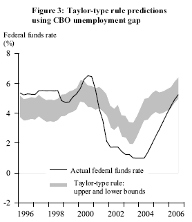
 Figure 3 plots the predicted level of the federal funds rate using a Taylor-type rule with a weight of 1.0 on the unemployment gap and a weight of 0.5 on the gap between actual and “desired” inflation. The unemployment gap is constructed using the less volatile CBO natural rate series. Inflation here is measured by the four-quarter change in the core PCE price index. In constructing the figure, two values for the desired inflation target are considered: 1% or 2%, defining what is often viewed as the Fed’s “comfort zone.” Two values for the long-run equilibrium real rate of interest are considered: 2% or 3%, reflecting typical empirical estimates.
As the figure shows, today’s 5.25% funds rate is slightly above the lower bound of the Taylor-type rule prediction, in contrast to the 2002-2004 period, when the funds rate was well below the lower bound. Still, the current stance of policy could be tightened by more than 100 basis points without exceeding the upper bound. Given the uncertainty about the true values of the inflation target, the equilibrium real interest rate, and the natural rate of unemployment, this exercise does not say definitively whether policy is too tight or too loose. According to the December 12 FOMC statement, “The extent and timing of any additional firming that may be needed to address [inflation] risks will depend on the evolution of the outlook for both inflation and economic growth, as implied by incoming information.”
Empirical estimates suggest that changes in the level of labor resource utilization, as measured by the unemployment gap, appear to be less useful for forecasting inflation than in the past. If anything, the Phillips curve predicts that core PCE inflation will drift upward over the next two years, because the prevailing unemployment rate is below estimates of the natural rate.
A weighted moving average forecast attempts to disentangle permanent versus temporary movements in the inflation rate. This decomposition is relevant to current policy discussions, because some of recent increase in core PCE inflation could be due to temporary factors, such as pass-through from high energy prices and a shift in the demand for rental housing that affects the shelter-cost component of core inflation. A retrospective evaluation of forecast accuracy shows that the weighted moving average forecast generally outperforms both the Phillips curve and a random walk forecast in predicting core PCE inflation one year ahead. The weighted moving average predicts that core PCE inflation will experience only a slight drop going forward because the current rate is close to the estimated inflation target.
Kevin J. Lansing
Senior Economist
[URLs accessed December 2006.]
Atkeson, A., and L.E. Ohanian. 2001. “Are Phillips Curves Useful for Forecasting Inflation?” FRB Minneapolis Quarterly Review (Winter) pp. 2-11.
Lansing, K.J. 2002. “Can the Phillips Curve Help Forecast Inflation?” FRBSF Economic Letter 2002-29 (October 4).
Lansing, K.J. 2006. “Time-Varying U.S. Inflation Dynamics and the New Keynesian Phillips Curve.” FRBSF Working Paper 2006-15.
USA Today. 2006. “Dissenting Fed Official Says Inflation a Risk.” September 6.
Williams, J.C. 2006. “Inflation Persistence in an Era of Well-Anchored Inflation Expectations.” FRBSF Economic Letter 2006-27 (October 13).
Opinions expressed in FRBSF Economic Letter do not necessarily reflect the views of the management of the Federal Reserve Bank of San Francisco or of the Board of Governors of the Federal Reserve System. This publication is edited by Anita Todd and Karen Barnes. Permission to reprint portions of articles or whole articles must be obtained in writing. Please send editorial comments and requests for reprint permission to research.library@sf.frb.org