Much recent discussion has suggested that the official real GDP data are inadequately adjusted for recurring seasonal fluctuations. A similar pattern of insufficient seasonal adjustment also affects the published data for a key measure of price inflation. Still, such residual seasonality in the published output and inflation statistics is unlikely to mislead Federal Reserve policymakers or adversely affect the setting of monetary policy.
Almost all economic data exhibit seasonal fluctuations—changes that occur around the same time each year due to such things as normal weather variation and holiday schedules. Because such variation obscures the underlying cyclical movements of the economy, most economic data are reported on a seasonally adjusted basis. Recently, a number of commentators have argued that the seasonal adjustment of real GDP by the Bureau of Economic Analysis (BEA) is incomplete and understates growth early in the year (see, for example, Rudebusch, Wilson, and Mahedy 2015). Indeed, since 1990, average real GDP growth has been significantly slower during the first three months of each year than in the subsequent quarters. Such “residual seasonality” in the published seasonally adjusted real GDP data should be taken into account when assessing the state of the economy. Accordingly, the very weak readings on real GDP for the first quarter of this year have been a concern to Federal Reserve policymakers as they try to discern whether the sluggish reported growth reflects residual seasonality or more fundamental factors (Yellen 2015).
Thus far, the analysis of residual seasonality has only focused on real GDP data. However, a key measure of prices—the price index for personal consumption expenditures (PCE)—is also seasonally adjusted by the BEA using the same methodology that it uses to construct GDP. As a result, it would not be surprising if the PCE price data were also plagued by residual seasonality. Such a misstatement could be particularly problematic because the PCE price index is widely used to assess underlying inflationary trends—particularly by Fed policymakers. Furthermore, the “core” version of this price index, which excludes volatile energy and food prices, has grown notably faster so far this year than it did last year. As one reporter (Hilsenrath 2015) noted: “Consumer prices, excluding food and energy, rose at a 1.8% annual rate in the second quarter. That is below the Fed’s 2% target but firmer than earlier months and firmer than many private analysts expected. It thus helps Fed officials gain confidence that inflation is stabilizing and could be poised to inch higher from low levels.”
This Economic Letter considers how much confidence policymakers can have in the signals from recent data in light of concerns about residual seasonality. We uncover significant residual seasonality in the published data on inflation and real GDP. Still, we argue that the potential adverse impact of residual seasonality on monetary policy is likely to be small.
Residual seasonality in core PCE inflation
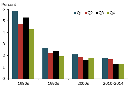
We investigate residual seasonality in core PCE inflation using the approach of Rudebusch et al. (2015). Figure 1 shows the average core PCE inflation rate by calendar quarter for each decade back to the 1980s—where inflation is measured as the three-month annualized percent change as of the last month of each quarter. For several decades, inflation has tended to be higher in the first half of the year than in the second half. This pattern has been especially evident during the past five years, when core PCE inflation averaged a little less than 2% in the first half of the year but closer to 1¼% in the second half.
Figure 1
Average core PCE inflation by quarter
Note: Seasonally adjusted 3-month percent change at annual rate.
This residual seasonality in aggregate inflation is not surprising given that the seasonal adjustment methodology for prices is similar to that for GDP. The BEA seasonally adjusts prices at a very disaggregated level and then combines the adjusted individual series to produce the top-line numbers. This granular, bottom-up method does not guarantee that the resulting aggregate series will be free of residual seasonality. To remove any remaining seasonality, we applied a second round of seasonal adjustment to the BEA’s seasonally adjusted core PCE price measure. Specifically, we apply the same seasonal adjustment procedure that the BEA uses—the Census Bureau’s well-known X12-ARIMA statistical filter—to the core PCE price index from the first quarter of 1960 through the second quarter of 2015 using monthly price levels at the end of each quarter.
Figure 2
Changes to core inflation by quarter from a second seasonal adjustment
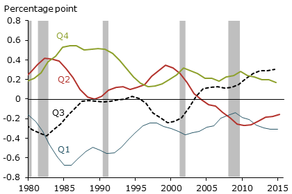
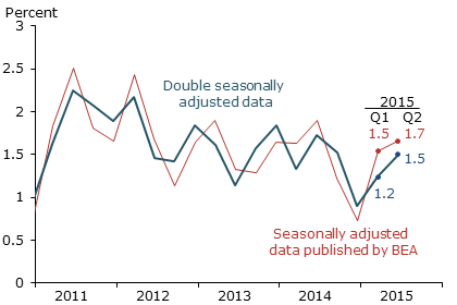
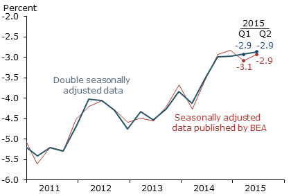
This technique provides seasonal adjustment factors that differ for each quarter and vary over time, as shown in Figure 2. These seasonal factors show the size of a second seasonal adjustment correction to the published three-month annualized core PCE inflation. If there were no residual seasonality, then the seasonal factors would all be zero. Instead, these factors are sizable and statistically significant. They show that reported inflation was probably overstated so far this year. The adjustments lower the published inflation series by about 0.3 and 0.2 percentage point in the first and second quarters of this year, respectively. To illustrate this correction, Figure 3 shows the recent inflation rate—both the BEA’s seasonally adjusted data in red and our double seasonally adjusted version in blue. The application of a second round of seasonal adjustment implies inflation of 1.2% in the first quarter and 1.5% in the second quarter, markedly lower than the inflation rates in the published data. Conversely, later this year, published inflation data are projected to be understated by the same amount.
Figure 3
Three-month core PCE inflation at an annual rate
Source: BEA and authors’ calculations.
Residual seasonality in real GDP growth
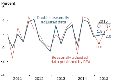
Rudebusch et al. (2015) found significant evidence of residual seasonality in the seasonally adjusted GDP data. Their second round of seasonal adjustment pushed the annualized real GDP growth rate 1.6 percentage points higher in the first quarter of this year. In July, the BEA released updated GDP data back through 2012 as part of its annual revision of the national income and product accounts. In this revision, the BEA implemented new procedures—within the overall constraints of its bottom-up methodology—to mitigate residual seasonality (see McCulla and Smith 2015). To evaluate the effect of the BEA’s annual revision, we applied a second round of seasonal adjustment to the updated GDP data. Figure 4 shows real GDP growth as currently published and a double seasonally adjusted version. The double adjusted series still indicates much faster growth in the first quarter of this year and a bit slower growth in the second quarter. Comparing these results to Rudebusch et al. (2015) suggests that the BEA updates were able to reduce recent residual seasonality in real GDP by about 20%.
Figure 4
Quarterly GDP growth at an annual rate
Source: BEA and authors’ calculations.
Will residual seasonality affect monetary policy decisions?
Assuming Fed policymakers were unaware of the residual seasonality in the published inflation and GDP data, to what extent could it mislead them in making monetary policy decisions? We examine this issue through the lens of simple monetary policy rules, which are often used as benchmarks for setting the fed funds rate—the short-term interest rate relevant for U.S. monetary policy.
For example, a standard policy rule response adjusts the funds rate by 1½ percentage points upwards or downwards, respectively, for every 1 percentage point increase or decrease in inflation. Therefore, if residual seasonality pushed inflation up by ¼ percentage point, then the rule would recommend that the funds rate should be almost ½ percentage point higher. Such policy rules that respond to quarterly changes in inflation are described by Rudebusch (2002) and Chen, Cúrdia, and Ferrero (2012). In these cases, residual seasonality could cause notable funds rate fluctuations and volatility—and perhaps premature liftoff from a zero lower bound in certain circumstances. Still, over the course of a year, as the overstatement and understatement of the published economic variables balance out, the average annual funds rate and stance of monetary policy would be unaffected. Furthermore, most policy rules reflect the usual practice of real-world policymakers so that monetary policy recommendations are based on year-over-year rather than quarterly changes in economic variables. For example, the balanced-approach policy rule in Yellen (2012) adjusts the funds rate in response to the four-quarter percent change in the PCE price index. Such temporal averaging over the seasonal cycle also eliminates the effects of residual seasonality on monetary policy.
Figure 5
Quarterly output gap
Source: BEA, Congressional Budget Office, and authors’ calculations.
Moreover, rather than relying on output growth, monetary policy rules are usually specified in terms of the output gap—the percent deviation of actual real GDP from potential GDP. The residual seasonality in GDP growth will also show through to the output gap, but in a greatly attenuated form. Figure 5 shows the published and double seasonally adjusted output gaps using the same underlying GDP data from Figure 4 and the Congressional Budget Office’s estimate of potential output. The sizable residual seasonality in output growth has a smaller apparent effect on the output gap because the former is reported at an annual rate, which exaggerates the effect. In the first quarter of this year, the published output gap is only 0.2 percentage point wider than the double seasonally adjusted version, so using the balanced-approach policy rule, this would imply a first-quarter funds rate that is too low by 0.2 percentage point. Again, this small effect would be unwound later this year.
Although the adverse effects of residual seasonality on monetary policy are likely to be fairly modest, they do illustrate one reason why central bankers are loath to follow any mechanical rule where the stance of monetary policy depends on only two economic variables. Any economic variable is inevitably imperfectly measured, so policymakers generally see advantages to using judgment and analysis to weigh a wide range of indicators. For example, at the beginning of this year, a variety of sources—including separate readings on employment and industrial production as well as anecdotal business reports—contradicted indications from the official GDP statistics that the economic recovery was faltering. Taking a broad-based, nuanced approach to setting policy can mitigate any adverse effects of residual seasonality.
Conclusion
Because the BEA adjusts for seasonal movements at a disaggregated level, the published seasonally adjusted PCE price inflation and real GDP data both exhibit calendar-based fluctuations—that is, residual seasonality. After we apply a second round of seasonal adjustment directly to the published aggregates, we estimate that inflation was lower and economic growth was faster during the first half of this year than currently reported in the published data. However, policymakers realize that any single piece of data, even a comprehensive measure like GDP, has to be taken with a grain of salt. Because of this, they are unlikely to be misled by the transitory statistical noise arising from residual seasonality.
Glenn D. Rudebusch is director of research and executive vice president in the Economic Research Department of the Federal Reserve Bank of San Francisco.
Daniel J. Wilson is a research advisor in the Economic Research Department of the Federal Reserve Bank of San Francisco.
Benjamin Pyle is a research associate in the Economic Research Department of the Federal Reserve Bank of San Francisco.
References
Chen, Han, Vasco Cúrdia, and Andrea Ferrero. 2012. “The Macroeconomic Effects of Large-Scale Asset Purchase Programmes.” The Economic Journal 122(564), pp. 289–315.
Hilsenrath, Jon. 2015. “Grand Central: GDP Data Support a Soon-and-Slow Rate Hike Strategy.” Real-Time Economics blog, The Wall Street Journal online, July 31.
McCulla, Stephanie H., and Shelly Smith. 2015. “Preview of the 2015 Annual Revision of the National Income and Product Accounts.” Bureau of Economic Analysis, Survey of Current Business 95 (June), pp. 1–8.
Rudebusch, Glenn D. 2002. “Assessing Nominal Income Rules for Monetary Policy with Model and Data Uncertainty.” The Economic Journal 112 (April), pp. 402–432.
Rudebusch, Glenn D., Daniel J. Wilson, and Tim Mahedy. 2015. “The Puzzle of Weak First-Quarter GDP Growth.” FRBSF Economic Letter 2015-16 (May 18).
Yellen, Janet L. 2012. “Perspectives on Monetary Policy.” Speech at the Boston Economic Club Dinner, Boston, MA, June
Yellen, Janet L. 2015. “Semiannual Monetary Policy Report to the Congress.” Testimony before the Committee on Financial Services, U.S. House of Representatives, Washington, DC, July 15.
Opinions expressed in FRBSF Economic Letter do not necessarily reflect the views of the management of the Federal Reserve Bank of San Francisco or of the Board of Governors of the Federal Reserve System. This publication is edited by Anita Todd and Karen Barnes. Permission to reprint portions of articles or whole articles must be obtained in writing. Please send editorial comments and requests for reprint permission to research.library@sf.frb.org