Investors have a hard time accounting for uncertainty when calculating how much risk they are willing to bear. They can use economic models to project future earnings, but many models are misspecified along important dimensions. One method investors appear to use to protect against particularly damaging errors in their model is by projecting worst-case scenarios. The responses to such pessimistic predictions provide insights that can explain many of the puzzles about asset prices.
As any would-be investor will attest, asset markets are difficult to understand. Economists share this confusion. Even with the benefit of hindsight and exhaustive analysis, there are many puzzling patterns in asset price data that are challenging to explain with standard economic models. Why do investors demand such high average returns to bear stock market risk? Why do stock prices gyrate so much, relative to dividends? Why are stock returns predictable despite the common intuition that they should be unpredictable? Why do investors jump on the bandwagon and overextrapolate from a run of high returns that they will earn further high returns in the future?
In this Economic Letter I discuss recent research by Bidder and Dew-Becker (forthcoming) that examines these puzzles. We begin with a framework in which investors doubt their model of the economy and consider alternative views of the world when making investment decisions. Because of their simplicity, economic models only broadly capture the actual economy and are misspecified along important dimensions. Faced with this uncertainty, investors try to protect against particularly damaging errors in their model. This Letter shows that attempting to protect against worst-case scenarios can lead investors to behave in such a way that explains many of the puzzles about asset prices.
Uncertainty
Nobody knows precisely how the world works. Nevertheless, people continually make decisions, so they must have in mind some benchmark model of the world. But what model? If the world is so complicated that phenomena relevant to a person’s economic welfare cannot be captured by a restricted set of rules based on limited data, it’s not clear how someone would decide on a model or how to use it, given the presumption that it is misspecified in some unknown way.
To account for this, Bidder and Dew-Becker (forthcoming) assume that investors use a pessimistically distorted version of the benchmark model to forecast future consumption and dividends and ultimately to price stocks. This pessimistic approach is characteristic of various methods of decisionmaking and forecasting in ambiguous situations (Gilboa and Schmeidler 1989 and Hansen and Sargent 2008).
Intuitively, when faced with profound uncertainty, it is natural for investors to try to limit their downside risk over a set of models, rather than try to identify optimal behavior for a single one. By envisaging painful misspecifications in the benchmark, an investor makes decisions that will perform reasonably well, even if the benchmark is wrong. Balancing between pain and plausibility results in a particular “worst-case” alternative model. When considering which assets to buy, the investor then makes decisions as if this model, rather than the benchmark, describes the economy.
Seeking a worst-case model
What determines the worst case? Bidder and Dew-Becker’s model describes how dividends and investors’ consumption vary randomly over time. The fluctuations in dividends are modeled as exaggerated versions of those in consumption. This is a simple way to capture the idea that dividends are procyclical—they tend to rise in economic expansions and fall during contractions—but are much more volatile than consumption. This connection between dividends and consumption is what makes stocks risky: They typically pay off poorly when an investor faces a downturn or expects weak conditions in the future. So, investors may want to pay particular attention to models that exaggerate these risk tendencies.
It is useful to think of a model as capturing how surprises today about consumption and, therefore, dividends carry into the future. If their effects die out quickly then there is little news about the distant future contained in the surprise. If the effects persist, however, this can provide information about both the current period and many future periods. For example, surprises could arise from unexpected business announcements or unanticipated changes in the broader economy.
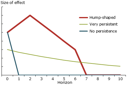
Figure 1 illustrates how models may differ in terms of what information is contained in surprises. Each line indicates how a surprise today changes expectations of consumption growth at different horizons in the future. The height of the line captures the size of the change and the horizon increases from left to right, with a horizon of zero indicating the current period. Some models, like the blue line, might imply that a surprise contains no news for future periods, so the line drops to zero immediately after the initial period. Other models might imply that a surprise has moderate implications for the immediate future, more for periods further in the future, but none beyond a particular horizon. In this case, the line has a hump shape initially, but then drops to zero, as shown by the red line. Finally, the green line indicates a model that has a relatively small impact in the current period, starting out lower than the other two lines, but features very long-lived effects, such that the line is still above zero even beyond the horizons plotted in the figure. These lines are referred to as “impulse responses,” and the point at which they reach zero is called their “order.”
Figure 1
Possible model responses of growth expectations to shock
Bidder and Dew-Becker suggest that an investor who is profoundly uncertain of how the world works probably doesn’t know the size or shape of the impulse response or even its order. In this case, it is natural to think the investor would allow for a wide range of possible outcomes and thus a broad class of models.
However, given a realistic span of data, there are only enough observations for the investor to estimate a simple benchmark model. Nevertheless, Bidder and Dew-Becker assume that the investor intends to develop a more complicated model as more data become available. This approach to estimation yields a benchmark model and also provides a basis for assessing the plausibility of alternative models.
Finding the worst case
Consider a simple economy that features no persistence in consumption growth. In line with the actual economy, assume that investors’ estimated benchmark model also displays no persistence, but that they doubt this model.
In Figure 2, the benchmark model is captured by the blue line, which shows the expected response of consumption growth to a shock. Consumption growth rises initially in response to the shock and falls back to zero afterward. The figure also shows the equivalent response under the worst-case model (green line), which is particularly interesting. It features shocks with essentially the same initial effect as under the benchmark, but the effects persist longer. Most important, while the effects on future expectations are small in any given period, they die out very slowly so that their combined effect becomes substantial.
Figure 2
Response to shock in benchmark and worst-case models
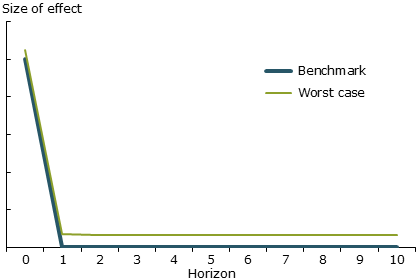
Because the impact of the worst case is similar to the benchmark and deviations from the benchmark at any given horizon are small the worst-case model is difficult to distinguish from the benchmark in practice. Consequently, investors will perceive the worst-case scenario as plausible and therefore worth worrying about. If the worst case were wildly different from the benchmark model the investor would dismiss it as unrealistic.
Intuitively, investors fear a shock that spreads its effects evenly across many future dates—a shock that will effectively last the rest of their lives. Such models are often referred to as “long-run risk” models, as proposed by Bansal and Yaron (2004). However, long-run risks are very difficult to detect and characterize. Indeed, their existence has even been questioned (Beeler and Campbell 2012). However, in the Bidder and Dew-Becker model, long-run risk need not actually exist. It is sufficient that investors believe it is plausible and painful enough that it features in the worst case and influences how they price assets.
Empirical implications
Investors behave as though they are using the worst-case model to forecast consumption and dividends. This model implies that equity holdings will pay off badly in times when investors are particularly vulnerable—when their consumption is low and, given the exaggerated persistence under the worst case, they expect future consumption growth will also be low. Thus, according to the worst case, holding equities exposes the investor to considerable risk. As a result these investments will have substantial risk premiums—that is, they will have to generate higher returns to account for the risk involved—which is consistent with the actual data. The risk premiums therefore reflect not only investors’ aversion to risk but also uncertainty about what risks exist. Importantly, this allows Bidder and Dew-Becker to assume investors have a reasonable amount of risk aversion, in contrast to other research that incorporates excessively high risk aversion to generate high premiums.
As well as elevated premiums, the model generates volatile stock prices and predictable returns. These phenomena are connected. When a shock unexpectedly lowers consumption, and therefore dividends, investors behave as if this condition will persist. Consequently, they will be less willing to buy the asset because they expect lower future cash flows—reflecting the additional persistence of shocks under the worst case. The price of the asset must drop dramatically to clear the market, implying negative returns. The amplified price movements, which also occur after positive shocks, lead to extra volatility in returns.
Regarding predictability, recall that, although the agent wants to guard against the possibility of long-run risk, the true model of the economy is not subject to risks over the long run. In fact, cash flow shocks are not persistent. So while the stock price drops when a negative shock hits, it will typically drift upwards in subsequent periods as cash flows will not, on average, justify the expectations implied by the worst-case scenario.
Finally, it is worth noting that these results depend on the uncertain investor overextrapolating relative to what the benchmark would imply. There is a common belief that investors jump on trends and excessively project past performance into the future, as discussed in Fuster (2011) and Greenwood and Shleifer (2014). The Bidder and Dew-Becker model shows how this sort of behavior can be rationalized if investors are uncertain about the world and behave as though they are informed by the worst case. That is, the worst case suggests that a positive surprise today raises the probability of higher dividend growth in the future, so that dividends do exhibit a type of trend in the mind of the investor.
Conclusions
This Letter proposes a model for how investors behave in an environment of profound uncertainty. The long-run risk model developed in Bidder and Dew-Becker (forthcoming) uses a process for projecting consumption growth that is undesirable for investors but that still is plausible. The model is therefore sensible for uncertain investors to use to protect against the worst-case scenario, even if it does not depict a true model of the world. In using this method, investors behave in a way that is consistent with many of the puzzling asset pricing characteristics apparent in the data.
Rhys Bidder is an economist in the Economic Research Department of the Federal Reserve Bank of San Francisco.
References
Bansal, Ravi, and Amir Yaron. 2004. “Risks for the Long-Run: A Potential Resolution of Asset Pricing Puzzles.” Journal of Finance 59(4, August), pp. 1,481–1,509.
Beeler, Jason, and John Y. Campbell. 2012. “The Long-Run Risks Model and Aggregate Asset Prices: An Empirical Assessment.” Critical Finance Review 1(1), pp. 141–182.
Bidder, Rhys, and Ian Dew-Becker. Forthcoming. “Long-Run Risk Is the Worst-Case Scenario.” Forthcoming in American Economic Review. FRBSF Working Paper version.
Fuster, Andreas, Benjamin Hebert, and David Laibson. 2011. “Natural Expectations, Macroeconomic Dynamics, and Asset Pricing.” NBER Macroeconomics Annual 26(1), pp. 1–48.
Gilboa, Itzhak, and David Schmeidler. 1989. “Maxmin Expected Utility with Non-unique Prior.” Journal of Mathematical Economics 18(2, April), pp. 141–153.
Greenwood, Robin, and Andrei Shleifer. 2014. “Expectations of Returns and Expected Returns.” Review of Financial Studies 27(3), pp. 714–746.
Hansen, Lars P., and Thomas J. Sargent. 2007. Robustness. Princeton, NJ: Princeton University Press.
Opinions expressed in FRBSF Economic Letter do not necessarily reflect the views of the management of the Federal Reserve Bank of San Francisco or of the Board of Governors of the Federal Reserve System. This publication is edited by Anita Todd and Karen Barnes. Permission to reprint portions of articles or whole articles must be obtained in writing. Please send editorial comments and requests for reprint permission to research.library@sf.frb.org