
Understanding how rain, snow, and cold weather affect the economy is important for interpreting economic data. A new study uses county-level data to measure the effect of unseasonable weather on monthly U.S. employment. The resulting estimates quantify how the atypical weather this year explains some of the unexpected fluctuations in hiring at the national level.
Weather plays an obvious role in the economy. Snowstorms can make it harder for people to get to work or shop. Rain can also put a damper on retail shopping but typically is good for agriculture. Warm temperatures tend to spur outdoor recreation, but too much heat can raise cooling bills for homes and businesses.
Many of these economic effects of weather are regularly recurring seasonal patterns. The statistical agencies that measure economic activity such as job growth account for normal seasonal fluctuations. But the weather doesn’t always follow these smooth patterns. Aberrations like heat waves, severe snowstorms, excessive rainfall, and unusually mild winters can have immediate, and potentially lingering, impacts on local and even national economies. To help policymakers sort out how much current economic ups and downs are due to transitory weather blips rather than economic fundamentals, researchers are finding new ways to estimate how unexpected weather might tie into measures of economic activity. The estimates are then used to adjust those measures in real time to strip out the effects of unusual weather or, more precisely, the deviations of weather from seasonal norms.
In this Economic Letter, we discuss a new model developed in Wilson (2016) that uses monthly data from U.S. counties on weather and employment. Importantly, this approach accounts for variation in weather and its effects across narrow geographic areas, enabling more precise measurement than approaches that rely on broader geographic data. The results provide a rich quantitative understanding of the short-term effects of temperature, precipitation, and snowfall on employment growth in specific industries and regions.
We then plug real-time weather data by county and month into the model and add up the county-level effects to estimate monthly weather effects on national employment. We find that weather can help explain fluctuations in national employment, both historically and in real time. Applying this to employment changes over recent months shows that weather effects were especially important this past spring. In particular, the model suggests that the weak national employment gains in May 2016 can be attributed largely to unusually adverse weather in May following unusually favorable weather in February and March. These atypical weather patterns pulled some economic activity that normally would have occurred in May forward to earlier months.
Estimating local weather effects
Wilson (2016) estimates weather’s economic effects using regression analysis, a statistical technique common in economics. Specifically, the approach provides a way to estimate both contemporaneous—that is, within the same month—and delayed or “lagged” effects of weather on an economic outcome, in this case monthly employment growth. Importantly, the model accounts for the influence of other regular seasonal variations in a county’s employment growth, such as post-holiday retail employment declines in January combined with reductions in construction jobs in areas with harsh winters. This seasonal adjustment removes the effects of such factors, as well as the effects of typical weather for a given county and calendar month, allowing us to focus on the effects of weather deviations from seasonal norms.
Wilson draws on the vast amount of detailed local data on employment and weather available from various sources: for employment growth, monthly Census of Employment and Wages data from the Bureau of Labor Statistics (BLS) from January 1990 to December 2015, by county (3,108 counties) and by industry (10 broad private-sector industries and private all-industry employment); and for weather, daily weather station data from the National Oceanic and Atmospheric Administration (NOAA). Wilson follows the methodology of Ranson (2014) to build monthly weather measures by county based on the daily records from local weather stations.
The combined county-by-month data set on employment and weather consists of nearly 1 million observations for any given industry. The large number of observations makes it possible to estimate a very detailed model of how weather might affect employment. In particular, the model can estimate not only the dynamic effects of each weather variable—that is, how weather affects employment in the same month as well as in subsequent months—but also how these effects differ across industries and regions. The model also allows temperature effects to vary across seasons. For instance, unseasonably high temperatures in the winter are likely to have different economic effects than unseasonably high temperatures in the summer.
In the model, observations are weighted by county employment, so that observations from more populous counties have a greater influence on the estimates of the weather effects. This accounts for counties with larger populations having more weather stations nearby and thus more accurate weather measurements.
Figure 1 shows the results of estimating the dynamic effects of five weather variables on private nonfarm employment growth. The first variable is the average daily high temperature for the month, which is allowed to affect employment growth differently in each of the four seasons (panel A). The other four variables shown in panel B are average daily precipitation, average daily snowfall, the number of days the temperature exceeded 90 degrees Fahrenheit, and the number of days with a temperature below 30 degrees. Each group of bars shows the estimated coefficient on the contemporaneous variables and their values one month, two months, and three months earlier. The variables have been normalized by the standard deviations for the full sample, so these coefficients can be interpreted as the effect on local employment growth of a one-standard-deviation move in the indicated weather variable.
Figure 1
Short-run dynamic effects of weather on private nonfarm employment growth
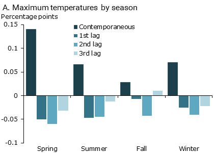
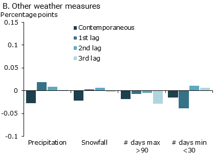
The model yields several interesting findings. First, panel A suggests local employment growth increases with the average temperature within the month. This is true in all four seasons but especially in the spring. However, the initial employment boost from temperature is largely transitory: Negative effects of lagged temperature lead to roughly zero cumulative effects over a four-month period. The pattern of the boost from higher temperatures in the current month, followed by a payback of reduced employment growth in the next two or three months, is especially pronounced for the spring and summer. Second, panel B shows that precipitation and snowfall have clear negative contemporaneous effects. But precipitation’s effect is offset by higher growth in the next three months, while snowfall’s four-month cumulative effect remains negative. Third, the frequency of very hot days in a month, holding the average temperature fixed, has a negative contemporaneous and cumulative effect on employment growth; this may reflect that extreme heat increases business operating costs, such as air conditioning, and could significantly dampen employment growth if it persists over several months. The frequency of very cold days, on the other hand, does not generally have significant effects.
It also is worth noting that Wilson (2016) finds that the effects of weather differ considerably across regions and industries. For instance, the most weather-sensitive industries generally are construction, natural resources and mining, and leisure and hospitality.
Adjusting national employment data for weather
The model estimates provide a prediction of how employment growth in any given county and month changes as a function of weather. Thus, we can use this model to ask what employment growth would have been had weather followed historical norms for that county and month. The difference between actual employment growth and this normal-weather scenario gives us an estimate of the total weather effect for that county and month.
We add up the county effects, accounting for the relative size of each county’s employment base, to estimate the effect of weather on national employment growth for the latest and previous months. Because the NOAA releases weather data daily with only a one-day lag, we can calculate national monthly weather effects within a few days of the end of a month—virtually in real time.
As a basis for comparison, we start with the BLS official level of private nonfarm employment in November 2015. We then apply the estimated weather growth effects from Dec. 2015 through the latest month of employment data (currently August 2016) to get the implied weather-adjusted levels of employment. Finally, we calculate the month-to-month changes in adjusted employment and multiply these changes by the private sector’s share of total nonfarm employment, currently 85%; we focus on the private sector because we assume government employment is not sensitive to weather. This calculation gives us an estimate of weather-adjusted total nonfarm employment change.
Figure 2 shows the resulting estimates for March through August of this year. (We will update our estimates for weather-adjusted employment change to reflect the most recent six months of data shortly after the official BLS employment report each month.) The first set of bars in Figure 2 shows the official BLS data on monthly employment change, which are not adjusted for weather. The second set shows weather-adjusted employment change based on estimates from our county model. For comparison, the third set shows estimates of weather-adjusted employment change from the Brookings Institution, based on the model of Boldin and Wright (2015), which uses national time-series data on weather and employment. Their model allows for the effect of weather in the current month and one subsequent month, though it imposes a constraint that the current and lagged effects cancel out.
Figure 2
Weather-adjusted employment change by month
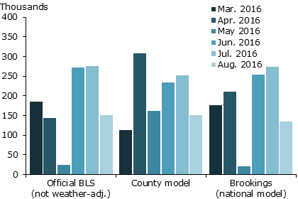
Source: Bureau of Labor Statistics, Brookings Institution, and authors’ calculations.
Weather effects over the three later months in the figure appear relatively minor. This is driven by the fact that this summer’s weather was fairly typical on average across the country. In contrast, weather effects during the spring were quite large according to the estimates using the county model. In particular, the model attributes much of the weakness in May’s official employment number to weather. In fact, accounting for a decline of 35,000 jobs attributable to the Verizon strike, the county model suggests that net job gains in May would have been 196,000. This is very close to the model’s average for weather-adjusted employment changes from March through May.
The county model results for May contrast with those from the Brookings national model. A look “under the hood” of the estimated county model and recent weather data explains why. Recall that the county model estimates that employment growth in the spring and summer is positively affected by current temperatures but negatively affected by temperatures in the prior three months. It turns out that May was unusually cold nationally, while February and March were especially warm. Hence, May employment growth appeared to be hampered by a kind of double whammy: May’s economic activity was held down by an unusual cold spell, and the warm February and March temperatures pulled some employment forward that normally would have occurred in May.
Conclusion
The estimates explored in this Letter suggest that weather can help explain recent fluctuations in employment, both at the local and national levels. This is not to say that weather is a dominant factor in monthly job fluctuations. Indeed, Wilson (2016) shows that weather explains only a small fraction of the variation in national monthly employment growth. The bulk of the variation is driven by the underlying strength of the labor market and unpredictable factors such as work stoppages in specific industries. Nonetheless, weather often does have important effects. This suggests that empirical models of weather effects can be useful to give policymakers a cleaner read on the economy’s underlying strength.
Catherine van der List is a graduate student in economics at the University of British Columbia and a former research associate in the Economic Research Department of the Federal Reserve Bank of San Francisco.
Daniel J. Wilson is a research advisor in the Economic Research Department of the Federal Reserve Bank of San Francisco.
References
Bloesch, Justin, and Francois Gourio. 2015. “The Effect of Winter Weather on U.S. Economic Activity.” FRB Chicago Economic Perspectives.
Boldin, Michael, and Jonathan H. Wright. 2015. “Weather-Adjusting Economic Data.” Brookings Papers on Economic Activity, Fall.
Ranson, Matthew. 2014. “Crime, Weather, and Climate Change.” Journal of Environmental Economics and Management 67(3), pp. 274–302.
Wilson, Daniel J. 2016. “The Economic Effects of Weather: Evidence from Big Data on Small Places.” FRB San Francisco Working Paper 2016-21.
Opinions expressed in FRBSF Economic Letter do not necessarily reflect the views of the management of the Federal Reserve Bank of San Francisco or of the Board of Governors of the Federal Reserve System. This publication is edited by Anita Todd and Karen Barnes. Permission to reprint portions of articles or whole articles must be obtained in writing. Please send editorial comments and requests for reprint permission to research.library@sf.frb.org