

The well-known Phillips curve describes inflation as a persistent process that depends on public expectations of future inflation and economic slack, a measure of how stretched the economy’s resources are. The role of each component has changed over time. In particular, maintaining the public’s expectations that the Federal Reserve is committed to an inflation target of 2% has grown in importance over the slack component, in part because realigning expectations is costly to undo. Such considerations are important as the Federal Reserve evaluates its future policy options.
The U.S. economy is running well above long-term sustainable growth according to many measures. The Congressional Budget Office says output “is projected to grow slightly faster than its maximum sustainable level this year” (CBO 2019). This higher growth means that resource constraints are likely to place increasing limits on the expansion. The unemployment rate is also near historic lows, averaging just 3.8% in the second half of 2018 as the growth in job openings outpaces the number of people seeking work. Together these measures indicate that there is limited economic slack. This situation would usually be associated with inflationary pressures on prices and wages. Yet, core inflation measured using personal consumption expenditures without food or energy, or core PCE, was 2% in the third quarter of 2018—the Federal Reserve’s inflation target. Moreover, recent labor compensation measures are consistent with this level of inflation and current measures of productivity, suggesting that wage pressures are well contained. So where is inflation headed?
In this Economic Letter we rely on a well-worn framework, the Phillips curve, to examine the dynamics of inflation. We focus on one version of the Phillips curve that relates inflation to economic slack, past inflation, and expectations about its future readings, among other factors. Our estimates show that, in the years since the Great Recession, inflation has been driven primarily by public expectations of future inflation rather than by economic slack. The vanishing relationship between slack and inflation is known in economics as a “flattening” of the Phillips curve.
The increased importance of inflation expectations exposes new risks to standard monetary policy practice. In particular, it suggests that conducting policy consistently to keep expectations well-anchored to the target is key to avoiding large swings in inflation. When policy is set consistently, the public discounts deviations of the unemployment rate from its natural rate and of inflation from its target as transitory.
The logic of the Phillips curve
The Phillips curve is a standard model of inflation dynamics and commonly describes current inflation as a function of three components: economic slack, past inflation, and expectations of future inflation. The more stretched the economy’s resources are, the more the pressure for prices to rise. In addition, inflation tends to respond slowly to fluctuations in economic activity that affect overall slack. This means that inflation is persistent, depending partly on past inflation, thus creating a feedback loop. Moreover, if people believe the central bank is conducting monetary policy to keep inflation at target, they may discount such fluctuations and instead use the targeted level of inflation as their reference point.
Past analyses suggest that patterns in historical inflation reflect all three components of the Phillips curve, but with variation over time. Dependence on economic slack and considerable inflation persistence have dominated much of the postwar experience. More recently however, and especially since the Great Recession, the expectations component has become the dominant factor explaining inflation dynamics (International Monetary Fund 2013 and Coibion and Gorodnichenko 2015). Researchers have argued that the low and stable rates of inflation experienced since the mid-1980s came with a decline in persistence and a bigger role for expectations about future inflation (Williams 2006).
Inflation dynamics in recent times
Figure 1 shows the decline in the slope of the Phillips curve in the past 40 years. The figure reports the relationships between headline consumer price index (CPI) inflation and economic slack during the two most recent decades and, as a reference, during the preceding 20 years. We measure economic slack using the unemployment gap, that is, the difference between the current unemployment rate and its natural rate as measured by the CBO. The natural rate of unemployment is the rate that would prevail in an economy at full productive capacity. The unemployment gap is positive when the economy’s resources are underutilized, and it is negative otherwise, making it a standard measure of economic slack.
Figure 1
Link between inflation, economic slack has weakened
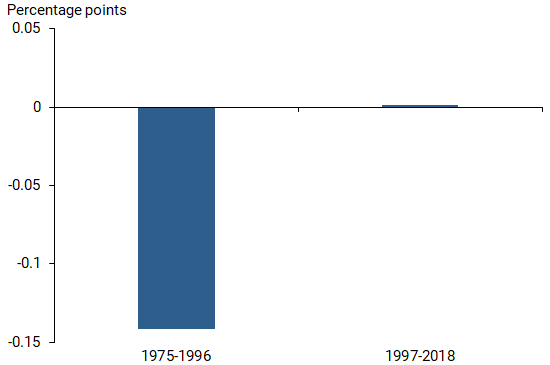
Note: Weight on unemployment gap in Phillips curve.
The evidence depicted in Figure 1 is rather striking. The link between inflation and economic slack has weakened substantially—the bar has almost vanished—during the most recent 20 years. Today, most analysts agree that the Phillips curve is essentially flat.
Given the evidence in Figure 1, the next step is to examine whether and how the Great Recession contributed to the change in the Phillips curve. We estimate the Phillips curve more formally for the 10 years preceding and since the Great Recession. We model inflation as a function of economic slack, lagged inflation, and expectations of future inflation. We continue to measure slack using the unemployment gap, we rely on headline CPI as our measure of inflation, and we use the one-year-ahead CPI inflation forecast from the Survey of Professional Forecasters (SPF) as our metric for inflation expectations. In addition, we include oil prices to account for inflation pressures coming from factors outside of the Federal Reserve’s control. Oil prices are useful for this because they are determined in international markets and, therefore, do not react to U.S. monetary policy.
Figure 2 summarizes our statistical analysis of the contributions from the three components for the periods before and after the Great Recession. As anticipated by Figure 1, the first pair of bars, the “slope” of the Phillips curve—which measures the influence of economic slack on inflation—is close to zero in both samples; changes in economic slack have had next to no effect on the dynamics of inflation before and after the Great Recession.
Figure 2
Contributors to Phillips curve changes before, after recession
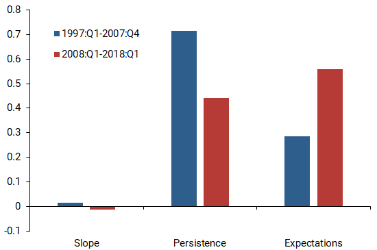
The second pair of bars in Figure 2 shows that inflation persistence has declined considerably, thus reducing the feedback loop somewhat. Currently, our estimates indicate that an unanticipated percentage point increase in inflation will raise inflation in the next quarter by about 0.45 percentage point. In contrast, prior to 2007, the effect on inflation would be about 0.71 percentage point.
Mirroring what has happened with persistence, the third pair of bars in Figure 2 shows that the contribution of future expectations has increased proportionately, almost doubling since the Great Recession. This increase implies that expectations now have a large effect on where inflation is headed.
Given the increasing importance of inflation expectations in determining current inflation readings, Figure 3 depicts the one-year-ahead measure of inflation expectations we use in our analysis. The figure shows that, despite some volatility, short-term expectations have fluctuated around the Fed’s 2% target, particularly since the Great Recession. Together with the fact that longer-term expectations have hovered near 2% (Nechio 2015) since the Fed’s announcement of its inflation objective in 2012, the evidence suggests that inflation expectations are well anchored.
Figure 3
One-year-ahead inflation expectations vs. Fed target
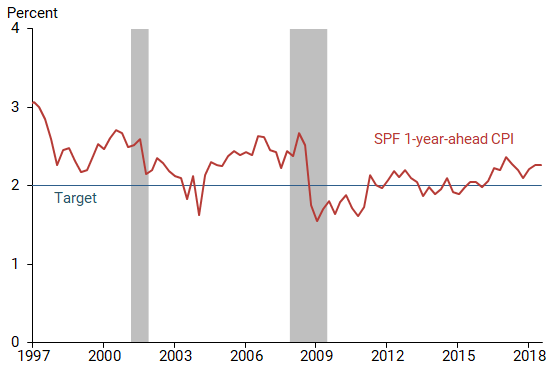
Note: Gray bars indicate NBER recession dates.
What could go wrong?
Estimates of the Phillips curve are just that, estimates. Moreover, the natural rate of unemployment is not directly observable. And the curve itself evolves over time, as Figure 1 shows. For all these reasons, it makes sense to stress-test our findings by considering three alternative scenarios. In the first scenario we ask what would happen if there were considerably less slack than currently measured by the CBO. In the second scenario, we examine what would happen if the Phillips curve became steeper. In the third and final scenario, we examine how changes in inflation expectations would modify the dynamics of inflation. Figure 4 summarizes the resulting net boost to inflation in each of these three experiments.
Figure 4
Estimated net boost to inflation in three scenarios
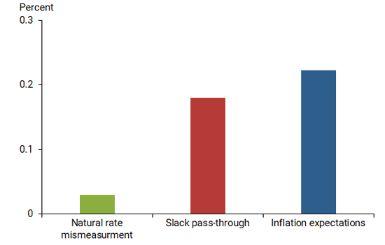
In the first scenario, suppose that the natural rate of unemployment were 2 percentage points higher than currently calculated. This may seem exaggerated. However, the natural rate can only be estimated, and our assumption happens to be just inside the range of possible values estimated from historical data (Watson 2014). Nevertheless, the contribution of economic slack to inflation is very small. Even if the unemployment rate truly were a full 2 percentage points further from its natural rate, the overall effect on inflation would be relatively small, less than a tenth of a percentage point, as the first bar in Figure 4 shows. This is a direct result of a flat Phillips curve.
Next, we reverse this experiment by instead increasing the impact of economic slack from essentially zero to 0.15, as it was in the 1975–1996 sample (Figure 1), while keeping the unemployment gap at its current reading. As the second bar in Figure 4 shows, this would result in a slightly larger boost to inflation than the previous scenario, somewhere in the neighborhood of an additional 0.13 percentage point, pushing inflation to 2.1%, still quite close to target.
In our final experiment, we consider what would happen if the short-term one-year-ahead expectations of future inflation drifted away from 2 to 2.4%, a value observed, for example, in the lead-up to the Great Recession. The third bar of Figure 4 shows that this scenario would translate to adding 0.22 percentage point to actual inflation, moving it to 2.2%.
Naturally, more than one scenario could take place at the same time. In fact, the more inflation deviated from target, the more we would expect such deviations to persist. For example, given that persistence is 0.5 from Figure 2, if inflation expectations crept up to 2.4% as in our second scenario, inflation could eventually reach 2.4% coincidentally via the feedback mechanism. Giving people a reason to doubt the central bank’s commitment to maintaining inflation near target is clearly costly.
Conclusion
Central banks try to neutralize fluctuations in demand through effective monetary policy. As a result, inflation dynamics today are primarily explained, not by economic slack, but by the public’s expectations that monetary policy will keep inflation close to the Federal Reserve’s target. Prolonged changes to inflation expectations thus pose the biggest risk to inflation. A failure to maintain inflation expectations around the target could greatly undermine the Federal Reserve’s ability to achieve stable prices—part of its dual mandate— in the future.
Òscar Jordà is vice president in the Economic Research Department of the Federal Reserve Bank of San Francisco.
Chitra Marti is a research associate in the Economic Research Department of the Federal Reserve Bank of San Francisco.
Fernanda Nechio is a research advisor in the Economic Research Department of the Federal Reserve Bank of San Francisco.
Eric Tallman is a research associate in the Economic Research Department of the Federal Reserve Bank of San Francisco.
References
Coibion, Olivier, and Yuriy Gorodnichenko. 2015. “Is the Phillips Curve Alive and Well After All? Inflation Expectations and the Missing Disinflation.” American Economic Journal: Macroeconomics 7(1), pp. 197–232.
Congressional Budget Office. 2019. “The Budget and Economic Outlook: 2019 to 2029.” Report, January.
International Monetary Fund, 2013. “The Dog that Didn’t Bark: Has Inflation Been Muzzled or Was It Just Sleeping?” World Economic Outlook, Chapter 3, April.
Nechio, Fernanda. 2015. “Have Long-Term Inflation Expectations Declined?” FRBSF Economic Letter 2015-11 (April 6).
Watson, Mark W. 2014. “Inflation Persistence, the Nairu, and the Great Recession.” American Economic Review 104(5), pp 31-36.
Williams, John C. 2006. “Inflation Persistence in an Era of Well-Anchored Inflation Expectations.” FRBSF Economic Letter 2006-27 (October 13).
Opinions expressed in FRBSF Economic Letter do not necessarily reflect the views of the management of the Federal Reserve Bank of San Francisco or of the Board of Governors of the Federal Reserve System. This publication is edited by Anita Todd and Karen Barnes. Permission to reprint portions of articles or whole articles must be obtained in writing. Please send editorial comments and requests for reprint permission to research.library@sf.frb.org