Does Ultra-Low Unemployment Spur Rapid Wage Growth?

By most measures, the U.S. labor market is currently quite strong, with several industries even experiencing labor shortages. The U.S. unemployment rate has steadily declined since the end of the Great Recession and ran below 4% in the second half of 2018. Many forecasters expect unemployment to fall further, even after factoring in the recent volatility in the financial markets and declines in stock prices. The median projection from the Federal Reserve’s Summary of Economic Projections (SEP) sees the unemployment rate hitting 3.5% by the end of 2019, a level not seen since 1969. Other labor market indicators, from broader measures of unemployment to job quit rates or the rate of job vacancy postings, have also been strong and point to a tight labor market. Strong demand for workers in a tight labor market should push up wages. Yet, while wage growth has increased since the end of the Great Recession, the increase has been surprisingly modest relative to the pace of labor market tightening.

The relationship between wage growth and labor market tightness is known as the (wage) Phillips curve: as the labor market tightens, wage growth tends to increase. Analyzing the variation across cities and over time, Leduc and Wilson (2017) found this negative relationship has flattened somewhat over time, which is consistent with the subdued pickup in wage growth nationally.

However, a number of analysts have suggested that the Phillips curve might not be strictly linear: a 1 percentage point decline in the unemployment rate when the labor market is especially hot triggers a bigger boost to wage growth than a 1 percentage point decline in normal times. Indeed, standard models of the labor market imply such nonlinearity (Petrosky-Nadeau and Zhang 2017). If this is true, we should expect wage growth nationally to rise sharply as the labor market continues to tighten.

In this Economic Letter, we reassess whether ultra-low unemployment rates cause sharp increases in wage growth using state-level data. Some other recent studies also have looked at this question. Nalewaik (2016) used national time series data and found no evidence of an economically meaningful nonlinearity. However, one might argue that national data have little power to answer this question because unemployment rates well below 4% have rarely been seen in the past 50 years.

By contrast, U.S. states regularly experience unemployment rates lower than 4%. Hence, in this Letter, we examine the relationship between wage growth and unemployment using state-level data. We go beyond finding simple correlations and use a statistical approach to identify the causal effect of unemployment rate changes on wage growth. We find little evidence of nonlinearities.

A first look at the data

One important challenge in assessing the wage Phillips curve is that the ultra-low national unemployment rates forecast for 2019 have been extremely rare over the past half-century. The last time the U.S. unemployment rate was as low as 3.5% was December 1969. For states, by contrast, unemployment rates around that level are not particularly rare: Figure 1 shows the distribution of state unemployment rates from 1991 to 2016.

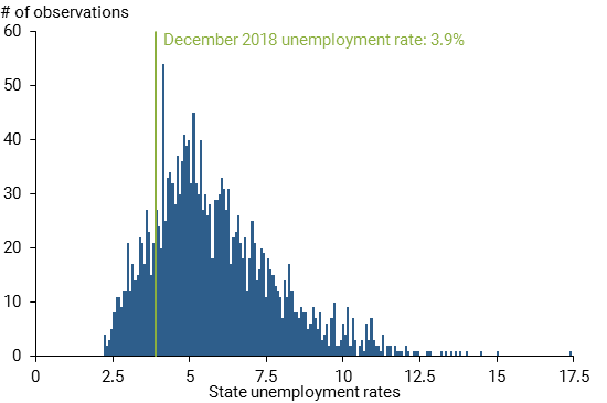
Given such ample variation in state unemployment rates, particularly at ultra-low levels, we can better assess whether wage growth rises sharply when labor markets turned hot, as is the case today.

We measure wage growth using individual-level data from the U.S. Census Bureau’s Current Population Survey (CPS), which collects demographic and employment data from about 60,000 households. For each head of household in the CPS, we calculate the average hourly earnings as the usual hourly earnings for both hourly and salaried workers including tips, commissions, and bonuses. We then calculate a weighted average of individual average hourly earnings for each state and year using CPS sampling weights to ensure a representative sample. Our measure of wage growth for each state and year is the year-over-year change in weighted-average hourly earnings.

Estimating a nonlinear wage Phillips curve

To examine the possibility that the wage Phillips curve is nonlinear, we look at the relationship between wage growth and the unemployment rate, allowing for the strength of this relationship to vary depending on the level of the unemployment rate. To do so, we first rank the state-by-year unemployment rates and divide them into four groups, with the lowest group representing unemployment rates below 4%. We then allow the slope to be different for each group in our estimate of the wage Phillips curve; formally, the shape is known as a piecewise-linear spline.

In estimating the wage Phillips curve, we adjust state wage growth and state unemployment rates by subtracting their national averages; this removes any influence of global or national factors, like monetary policy or oil prices, that vary by year. These so-called “year fixed effects” could affect both wage growth and the unemployment rate, making it harder to interpret the resulting correlation. We also adjust for “state fixed effects” — characteristics that lead to permanent differences between states—by subtracting state-specific averages across all years. In addition, growth in labor productivity can affect nominal wage growth. Since labor productivity can vary within a state over time, it would not be captured by state fixed effects, so we account for this separately. Finally, we control for lagged wage growth, which tends to be slow to adjust to changes in the labor market.

We first estimate the implied linear and nonlinear wage Phillips curve relationships using a standard statistical method known as ordinary least squares (OLS), shown in Figure 2. The linear relationship between wage growth and the unemployment rate (green line) assumes that the slope of the curve is the same regardless of the unemployment rate.

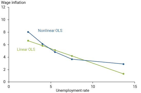
By contrast, the nonlinear version (blue line) allows the slope of the curve to change at different levels of the unemployment rate. The “knots” of this spline—that is, the levels of the unemployment rate where the slope of the Phillips curve is allowed to change—are indicated with circles. We grouped state unemployment rates into four groups: below 4.0%, between 4.0 and 5.5%, between 5.5 and 7.5%, and above 7.5%. We are most interested in the group below 4.0%, which represents ultra-low rates like those forecast nationally.

The OLS results point to a nonlinearity at unemployment rates around 7.5%. Specifically, the slope is significantly flatter when the unemployment rate is above 7.5% than it is below that level. This aligns with a similar finding by Kumar and Orrenius (2016). However, looking at lower unemployment rates like the ones forecast for the year ahead, we find no evidence of any economically meaningful nonlinearity. In particular, there is no evidence of a meaningful increase in wage growth as unemployment rates fall below 4%.

The OLS results, however, are just a correlational analysis. They do not necessarily reveal the causal effect of unemployment rate changes on wage growth; this information is important for policymakers who are concerned that stimulative monetary policy that boosts aggregate demand and lowers the unemployment rate could spark a sharp rise in wage growth and, in turn, inflation.

One main concern is that unobserved shocks to supply—that is, to production costs—could blur the findings by muting the negative relationship between wage growth and the unemployment rate. For instance, a shock that increases production costs could boost nominal wage growth via higher cost-of-living adjustments, while at the same time raising the unemployment rate via production cuts. Therefore, we adopt a strategy that specifically captures changes in the unemployment rate that are causally driven by shocks to aggregate demand only. We use a statistical method known as two-stage least squares (2SLS) to identify movements in the unemployment rate that are driven directly by changes in labor demand and then examine how those demand-driven movements influence wage growth.

To identify such demand-driven movements in unemployment rates, we use the fact that states differ substantially in their industry compositions due to their natural characteristics, making them relatively more or less sensitive to certain national or global shocks. For instance, some state economies are heavily dependent on foreign demand, making them—and their unemployment rates—especially sensitive to movements in the U.S. dollar. Changes in the value of the dollar lead to changes in the demand for states’ products that are sold abroad, affecting the unemployment rates of export-oriented states relatively more. Similarly, unemployment rates in states that extract oil and gas tend to be more sensitive to global movements in oil prices, and unemployment rates in agricultural states are sensitive to global movements in crop prices.

To isolate the demand-driven movements in unemployment rates, we first regress state-by-year unemployment rates on these three instruments, accounting for the same controls and “fixed effects” used in the OLS regression. Next, we reconstruct unemployment as only the part explained by these demand-driven shocks, throwing out anything else that could be due to supply. We then examine how these demand-driven movements in the unemployment rates affect wage growth.

We therefore construct three state-by-year variables, or “instruments,” that capture these differential demand shocks across states. The instruments are (1) the value of the dollar times the state’s average export share of GDP, (2) the Brent oil price times the state’s average oil and gas extraction share of GDP, and (3) the U.S. Department of Agriculture farm crop price index times the state’s average agricultural share of GDP.

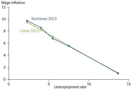
The implied linear and nonlinear wage Phillips curves from this estimation procedure are shown in Figure 3. We find that the nonlinear wage Phillips curve is approximately linear throughout the range of unemployment rates. In particular, there is no indication of any steepening in the slope as unemployment rates fall below 4%. We also see no indication of a flattening as unemployment rates rise above 7.5%, in contrast to the OLS results. The similarities between the estimated linear and nonlinear wage Phillips curves under the 2SLS approach suggests that the flattening seen in the OLS results may be due to unobserved supply-side factors that tend to be prevalent when labor markets are especially loose.

Conclusion

In sum, a careful look at the wage Phillips curve across states yields little evidence supporting the contention that wage growth sharply rises as the labor market reaches especially tight conditions. Of course, the current period may be different from the past. For instance, the typical pattern of local wage growth in a tight local labor market may differ when all other nearby labor markets are experiencing similar tightness, as is currently the case. As a result, geographical labor mobility—which can mute wage pressures in tight markets as workers are attracted to higher-wage areas—may be playing less of a restraining role. With this caveat in mind, given the historical experiences of states in recent decades, we do not foresee a sharp pickup in wage growth nationally if the labor market continues to tighten as many anticipate.

Sylvain Leduc is director of the Economic Research Department of the Federal Reserve Bank of San Francisco.

Chitra Marti is research associate in the Economic Research Department of the Federal Reserve Bank of San Francisco.

Daniel J. Wilson is vice president in the Economic Research Department of the Federal Reserve Bank of San Francisco.

References

Kumar, Anil, and Pia M. Orrenius. 2016. “A Closer Look at the Phillips Curve Using State Level Data.” Journal of Macroeconomics 47, Part A, pp. 84–102.

Leduc, Sylvain, and Daniel J. Wilson. 2017. “Has the Wage Phillips Curve Gone Dormant?” FRBSF Economic Letter 2017-30 (October 16).

Nalewaik, Jeremy. 2016. “Non-Linear Phillips Curves with Inflation Regime-Switching.” Finance and Economics Discussion Series 2016-078, Board of Governors of the Federal Reserve System.

Petrosky-Nadeau, Nicolas, and Lu Zhang. 2017. “Solving the Diamond-Mortensen-Pissarides Model Accurately.” Quantitative Economics 8(2), pp. 611–650.