
A key challenge for monetary policymakers is to predict where inflation is headed. One promising approach involves modifying a typical Phillips curve predictive regression to include an interaction variable, defined as the multiplicative combination of lagged inflation and the lagged output gap. This variable appears better able to capture the true underlying inflationary pressure associated with the output gap itself. Including the interaction variable helps improve the accuracy of Phillips curve inflation forecasts over various sample periods.
The Phillips curve is a key mathematical relationship that many economists use to predict where inflation is headed. The relationship presumes that near-term changes in inflation are partly driven by so-called gap variables. These may include the percent deviation of real GDP from potential GDP, known as the output gap, or the deviation of the unemployment rate from the natural rate of unemployment, known as the unemployment gap. Other drivers of inflation often included when estimating the Phillips curve are survey-based measures of expected inflation, lagged values of inflation, and special factors related to recent changes in oil or import prices. All else being equal, a larger output gap or a more negative unemployment gap implying a tighter labor market would predict rising inflation over the near term.
Numerous studies have found that estimated versions of the Phillips curve have become flatter over time, implying that the standard relationship has less predictive power for future inflation than it once had. This Economic Letter examines a potential way to improve Phillips curve forecasts of future inflation by including an interaction variable, defined as the multiplicative combination of lagged inflation and the lagged output gap. Multiplying the output gap by inflation rescales the gap to produce a new variable that appears better able to capture the true underlying inflationary pressure associated with the output gap itself.
Flattening of the Phillips curve
A long line of studies has examined the usefulness of the Phillips curve for forecasting inflation (see Lansing 2002, 2006 for a review). A typical finding is that estimated versions of the Phillips curve have become flatter over time, meaning that the regression coefficient on the gap variable—called the “slope” of the curve—has become smaller in magnitude, implying that the gap has less predictive power for future inflation. A completely flat Phillips curve, with a slope coefficient of zero, would imply that there is no relationship between the current value of the gap variable and future inflation. As one piece of evidence in this regard, the Great Recession from December 2007 through June 2009 delivered an extremely negative and persistent output gap together with soaring unemployment. But this episode did not produce a sustained decline in U.S. inflation, giving rise to the so-called “missing disinflation puzzle.”
To illustrate the basic idea of the flattening Phillips curve, Figure 1 plots the estimated slope coefficient from a series of 20-year rolling regressions, where quarterly data from the beginning of 1961 to the end of 1980 are used for the initial regression. For each 20-year sample period, the change in the inflation rate over the past four quarters is regressed on a constant term and the four-quarter lagged value of the output gap. This is a typical Phillips curve predictive regression along the lines of Stock and Watson (2018). For the inflation rate, I use the percentage change in the headline personal consumption expenditures price index (PCEPI) over the past four quarters. For the output gap, I use the percent deviation of real GDP from the real potential GDP series constructed by the Congressional Budget Office (CBO).
Figure 1
Estimated slope coefficient from 20-year rolling regressions
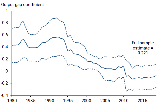
The estimated slope coefficient using the full sample of data from 1961 to 2018 is positive and statistically significant, consistent with the standard Phillips curve intuition. However, the rolling regressions show that the estimated slope coefficient declines over time and is not statistically significant from the first quarter of 2003 onward. Consistent with standard econometric practice for judging statistical significance, the dashed lines represent 95% confidence intervals for the estimated slope coefficient from each rolling regression. The estimated slope coefficient turns negative from the second quarter of 2010 onward. A negative slope coefficient turns the standard Phillips curve intuition on its head: a more positive output gap would predict lower, not higher, inflation over the near term.
Various hypotheses have been proposed to explain the declining slope coefficient. These include (1) a rise in the credibility of monetary policy that has served to anchor people’s inflation expectations, and hence inflation itself, to a value around 2%, (2) demographic shifts or other slow-moving forces that have contributed to mismeasurement of the gap variable, and (3) changes in technology and market competition that have limited the pass-through of wage growth to price inflation.
Improving Phillips curve forecasts
Identifying a more stable Phillips curve relationship would likely improve its usefulness for forecasting future inflation. Research along these lines has examined alternative gap measures (Ball and Mazumder 2011), alternative inflation measures (Mahedy and Shapiro 2017, Stock and Watson 2018, Ball and Mazumder 2019), alternative measures of expected inflation (Coibion and Gorodnichenko 2015), and alternative functional forms that allow for a nonlinear or time-varying relationship between the gap variable and future inflation (Ball and Mazumder 2011) Including a variable that measures how inflation and the output gap interact over time would fall into either the first or last category.
Figure 2 plots the CBO output gap versus the inflation-output gap interaction variable, defined as the multiplicative combination of the four-quarter PCE inflation rate and the CBO output gap. Both series are strongly procyclical—increasing during economic recoveries and decreasing during recessions. The correlation coefficient between the two series is 0.79. Given this very high correlation, I repeat the 20-year rolling regression exercise in Figure 1 using the interaction variable as the gap measure in place of the CBO output gap. Figure 3 shows that the resulting regression coefficient on the interaction variable remains positive from 1980 onward. Importantly, the estimated slope coefficient is reasonably stable over time and remains statistically significant for most of the 20-year sample periods.
Figure 2
Output gap versus inflation-output gap interaction variable
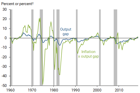
Note: Shaded areas represent NBER recession dates.
Figure 3
Estimated slope coefficient using interaction variable as gap
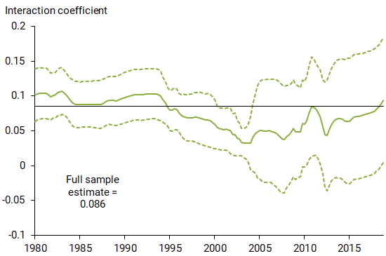
What explains the more stable slope coefficient in Figure 3 versus Figure 1? One explanation is that multiplying the output gap by inflation rescales the gap, producing a new variable that appears better able to capture the true underlying inflationary pressure associated with the gap itself. As Ball and Mazumder (2011) note, this is exactly what economic theory would predict for an environment where private-sector firms choose to raise their prices more frequently when inflation is higher. Periods of lower inflation, in turn, would induce less frequent price hikes. More generally, studies using machine learning techniques have found that allowing for interactions among a basic set of predictor variables can often improve forecasting performance. For example, Lansing, LeRoy, and Ma (2019) show that, while measures of consumer sentiment and stock return momentum are not helpful individually for predicting excess stock returns, a multiplicative combination of the two is a robust predictor of the excess stock return over the next month.
Inflation forecast comparisons
To better assess the predictive power of the inflation-output gap interaction variable, I compare inflation forecasts derived from a Phillips curve regression that omits this variable with an otherwise similar regression that includes it. In the first case, I regress the change in PCE inflation over the past four quarters on a constant term, the four-quarter lagged value of PCE inflation, and the four-quarter lagged value of the CBO output gap. In the second case, the regression equation also includes the four-quarter lagged value of the interaction variable. When estimated over the full sample of data from 1961 to 2018, the first regression accounts for about 21% of the variance of the dependent variable. The second regression accounts for 37% of the variance. While the in-sample fit of the second regression is much better, one may wonder about its out-of-sample forecasting performance. Oftentimes, a predictive regression that performs very well in-sample does poorly in out-of-sample forecasts because of “over-fitting.” This can happen when the estimated regression coefficients are too closely tailored to one particular set of data. However, this problem does not arise with the regression that includes the interaction variable.
Figure 4 plots the results of an out-of-sample forecast comparison. The two regression equations are each estimated using data from 1961 to 2007. The same equations are then used to forecast the four-quarter change in the PCE inflation rate for the period 2008 to 2018. Each forecast uses data that are lagged by four quarters relative to the forecasted date.
Figure 4
Comparing out-of-sample forecasts with interaction variable
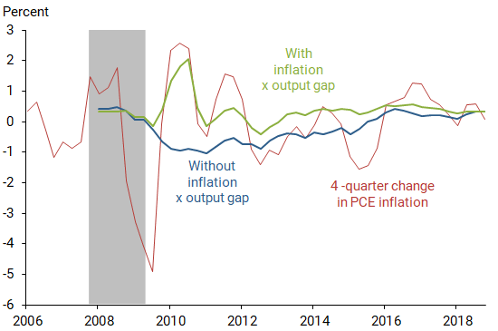
The out-of-sample forecasts from the second regression equation that includes the interaction variable substantially outperform those from the first regression equation that omits the interaction variable. Various forecast performance measures—including the root-mean-squared forecast error, the mean absolute forecast error, and the correlation coefficient between the forecasted value and the actual value—all favor the second regression equation. For example, the correlation coefficient between the forecasted and actual values in Figure 4 is 0.61 when the interaction variable is included versus –0.04 when this variable is omitted. A notable success of the second equation is that it correctly predicts a sharp jump in PCE inflation starting in the fourth quarter of 2009 following three consecutive quarters of negative inflation. This prediction arises because the interaction variable turns positive when negative inflation is multiplied by a negative output gap.
The forecasts constructed using the second equation also outperform a random walk inflation forecast, which presumes no change in PCE inflation over the next four quarters. In contrast, the forecasts constructed using the first equation underperform a random walk forecast. The out-of-sample forecasts from the second equation continue to outperform, albeit to a lesser degree, if the initial estimation period is from 1988 to 2007 instead of 1961 to 2007. The superior performance of the second equation also applies if I use core PCE inflation, which excludes volatile food and energy components, in place of headline PCE inflation. In this regard, it’s worth noting that the Fed’s 2% inflation target is formulated in terms of headline PCE inflation. Hence, the possibility of improving forecasts for this inflation measure may be of particular interest to policymakers.
Conclusion
Improving the accuracy of inflation forecasts is important for central banks that have pledged to achieve numerical inflation targets over a given time horizon. Research that explores alternative gap variables, alternative measures of inflation or expected inflation, and alternative functional forms all offer some promise to improve the usefulness of the Phillips curve for forecasting inflation. This Letter shows that including an inflation-output gap interaction variable can often help improve the accuracy of Phillips curve inflation forecasts, both in-sample and out-of-sample.
Kevin J. Lansing is a research advisor in the Economic Research Department of the Federal Reserve Bank of San Francisco.
References
Ball, Laurence, and Sandeep Mazumder. 2011. “Inflation Dynamics and the Great Recession.” Brookings Papers on Economic Activity, Spring 2011, pp. 337–405.
Ball, Laurence M., and Sandeep Mazumder. 2019. “The Nonpuzzling Behavior of Median Inflation.” National Bureau of Economic Research Working Paper 25512.
Coibion, Olivier, and Yuriy Gorodnichenko. 2015. “Is the Phillips Curve Alive and Well After All? Inflation Expectations and the Missing Disinflation.” American Economic Journal: Macroeconomics 7, pp. 197–232.
Lansing, Kevin J. 2002. “Can the Phillips Curve Help Forecast Inflation?” FRBSF Economic Letter 2002-29 (October 4).
Lansing, Kevin J. 2006. “Will Moderating Growth Reduce Inflation?” FRBSF Economic Letter 2006-37 (December 22).
Lansing, Kevin J., Stephen F. LeRoy, and Jun Ma. 2019. “Examining the Sources of Excess Return Predictability: Stochastic Volatility or Market Inefficiency?” FRBSF Working Paper 2018-14.
Mahedy, Tim, and Adam Shapiro. 2017. “What’s Down with Inflation?” FRBSF Economic Letter 2017-35 (November 27).
Stock, James H., and Mark W. Watson. 2018. “Slack and Cyclically Sensitive Inflation.” Working Paper, Harvard University.
Opinions expressed in FRBSF Economic Letter do not necessarily reflect the views of the management of the Federal Reserve Bank of San Francisco or of the Board of Governors of the Federal Reserve System. This publication is edited by Anita Todd and Karen Barnes. Permission to reprint portions of articles or whole articles must be obtained in writing. Please send editorial comments and requests for reprint permission to research.library@sf.frb.org