
History suggests that elevated values of the cyclically adjusted price-earnings (CAPE) ratio may indicate an overvalued stock market. A valuation model that uses a small set of economic variables can help account for movements in the CAPE ratio over the past six decades. One of these variables is a macroeconomic uncertainty index. Comparing the model’s prediction for the second and third quarters of 2020 to the 2008–2009 period suggests that investors have reacted to macroeconomic uncertainty very differently during the COVID-19 outbreak than they did during the financial crisis.
At the end of the third quarter of 2020, the Standard and Poor’s (S&P) 500 stock index closed 50% above the market low reached on March 23, 2020 during the early stages of the coronavirus disease 2019 (COVID-19) outbreak in the United States. The closing value for the third quarter was about 3% above levels that triggered some concerns about market overvaluation among participants at the January 28–29, 2020, Federal Open Market Committee meeting (Board of Governors 2020).
Making judgments about stock market valuation is a difficult endeavor. One metric, known as the cyclically adjusted price-earnings (CAPE) ratio, was originally developed by Campbell and Shiller (1998) to help gauge whether the stock market is overvalued.
This Economic Letter compares CAPE ratio levels in 2020 to those predicted by a simple valuation model that includes three macroeconomic variables—the “natural” real rate of interest, the growth rate of potential output, and an index of macroeconomic uncertainty. I find that the model’s predicted values for the second and third quarters are highly sensitive to the inclusion of the uncertainty index, which spiked upwards in March 2020 and remained elevated in June. Including the uncertainty index pushes the model’s predicted values for the CAPE ratio well below the actual ratios, suggesting possible overvaluation. Omitting the uncertainty index moves the predicted values closer to the actual ratios, pointing to a more reasonable valuation. Comparing the 2020 model predictions to those for 2008–2009 shows that elevated uncertainty appears to have had less negative effects on actual stock prices during the COVID-19 outbreak than during the financial crisis. This result highlights the difficulty of judging whether the stock market is overvalued and makes it hard to predict how investors will react to a future episode of elevated uncertainty.
The CAPE ratio and macroeconomic variables
Campbell and Shiller (1998) computed the CAPE ratio as the real, that is, inflation-adjusted, value of the S&P 500 divided by the real earnings of companies in the index averaged over the most recent 10 years. Averaging the denominator over a rolling 10-year window minimizes the impact of short-term earnings fluctuations on the ratio. Campbell and Shiller found that higher-than-average values of the CAPE ratio predicted lower-than-average future real returns on stocks over subsequent 10-year periods.
At the end of the third quarter of 2020, the CAPE ratio stood at 30.9. This value is below the prior peak of 32.6 in the third quarter of 2018, but it is about 51% above the long-term average of 20.5 from 1960 to present. To address whether these conditions might indicate an overvalued stock market, we can examine the degree to which recent movements in macroeconomic data can account for the latest values of the CAPE ratio.
In theory, the fundamental price of a stock is determined by the present value of expected future earnings distributions, or cash flows, that accrue to shareholders. The discount rate used in the present value calculation is comprised of a risk-free rate of return and a compensation for perceived risk, that is, a risk premium. All else being equal, a lower risk-free rate or a lower risk premium would imply that future cash flows are discounted less, causing the fundamental price to rise. Another variable that can influence the fundamental price is the expected growth rate of future cash flows, with higher growth implying a higher price.
One measure of the real risk-free rate of return is the natural real rate of interest, or “r-star.” Standard economic models imply that r-star is linked to households’ degree of patience, which influences their willingness to save, and to the expected growth rate of potential output, which influences the rate of return from saving. The same models imply that the growth rate of potential output determines the long-run growth rate of real cash flows from stocks.
Figure 1 shows the relationship between the CAPE ratio, an estimate of r-star from Laubach and Williams (2016), and the four-quarter growth rate of potential output from the Congressional Budget Office (CBO). The CAPE ratio exhibits a mostly upward-sloping trend, particularly since the early 1980s. R-star and potential growth both exhibit downward-sloping trends, but the decline in r-star is more pronounced, providing some rationale for the upward trend in the CAPE ratio.
Figure 1
CAPE ratio, natural real rate of interest, and potential growth
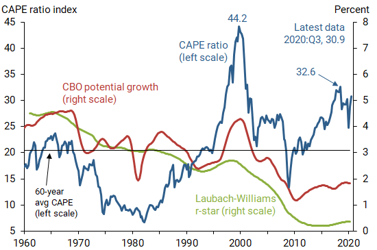
Source: Robert Shiller’s website.
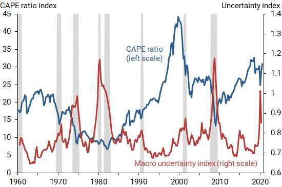
Uncertainty about the future path of the U.S. economy would be expected to influence uncertainty about future cash flows from stocks and thereby affect the risk premium required by investors. As a gauge of investors’ perceived risk, I consider an index of macroeconomic uncertainty constructed by Jurado, Ludvigson, and Ng (2015). The uncertainty index summarizes how difficult it is to forecast the near-term path of 132 separate macroeconomic variables using a joint statistical model of the U.S. economy. Higher values of the index indicate that the model’s three-month-ahead forecast errors have grown. The macroeconomic uncertainty index moves in the same direction as other measures of uncertainty that directly gauge stock market volatility.
Figure 2 shows the relationship between the CAPE ratio and the macroeconomic uncertainty index. As the economy heads into a recession, the uncertainty index starts rising. The uncertainty index in March 2020 is very high, albeit lower than the peak reached during the fourth quarter of 2008 during the financial crisis. The uncertainty index in June 2020 receded but remained elevated relative to pre-COVID-19 levels.
Figure 2
CAPE ratio and macroeconomic uncertainty
Actual versus fitted values for the CAPE ratio
I use a simple regression model to assess the ability of the macroeconomic variables to explain historical movements in the CAPE ratio. The model regresses the end-of-quarter CAPE ratio in logarithms on a constant, the Laubach-Williams estimate of r-star, the four-quarter growth rate of CBO potential output, and the end-of-quarter value of the macroeconomic uncertainty index. The explanatory variables are each lagged by one quarter relative to the CAPE ratio because third-quarter data are unavailable for r-star and the uncertainty index. Lansing (2017) estimates a similar regression model that includes core inflation as an explanatory variable but does not include the uncertainty index.
I estimate this model using data from 1961 through the third quarter of 2020. All of the explanatory variables are highly statistically significant. Consistent with standard asset pricing theory, higher values for r-star and the uncertainty index predict a lower CAPE ratio, while higher values for potential growth predict a higher CAPE ratio. The model’s explanatory power is quite good, accounting for 60% of the variance in the actual CAPE ratio over the past six decades. If the uncertainty index is omitted, the regression model accounts for only 51% of the variance in the actual CAPE ratio.
Figure 3 plots actual versus fitted values of the CAPE ratio, both with and without the uncertainty index included in the regression model. Including the uncertainty index (red line) helps the model fit the sharp drop in the actual ratio during the 2008–2009 financial crisis. The CAPE ratios predicted by this same model for the second and third quarters of 2020 are much lower than the actual ratios, suggesting overvaluation in the actual ratios. But if the uncertainty index is omitted (green line), the model predicts CAPE ratios in the second and third quarters that are closer to the actual ratios, suggesting more reasonable valuation.
Figure 3
Actual versus fitted CAPE ratios
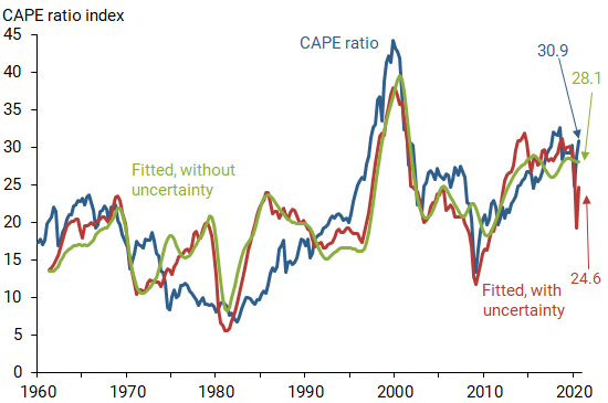
From Figure 3, it appears that investors are reacting to macroeconomic uncertainty very differently during the COVID-19 outbreak than they did during the financial crisis. Put another way, the uncertainty index appears less able to help explain the level of the CAPE ratio in recent data. Given this result, it is hard to predict how investors might react to a possible future increase in uncertainty.
CAPE ratio and investor expectations
Cochrane (2011) argues that a scenario of perceived overvaluation might instead be explained as a scenario where the risk premium required by rational investors is low. A lower risk premium would imply that future cash flows from stocks are discounted less, causing the fundamental price to rise. But going forward, the same lower risk premium would imply that rational investors should expect a lower rate of return from risky assets like stocks.
Examining investors’ expectations about future stock returns offers a way to distinguish between the two scenarios described by Cochrane. Rational investors with low risk premiums should expect low future returns from stocks after a sustained price run-up. In contrast, irrationally exuberant investors in the midst of a bubble should expect high future returns because they simply extrapolate from recent price changes. Evidence from investor survey data seems to support the second scenario.
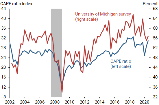
Figure 4 plots the CAPE ratio together with a gauge of investors’ expectations about future stock returns from a University of Michigan survey. The survey records investors’ perceived probability of an increase in stock prices over the next year. By Cochrane’s logic, rational investors should expect a lower probability of a price increase when the CAPE ratio is higher. But the survey data seem to show the opposite pattern: investors appear to expect a higher probability of a price increase when the CAPE ratio is higher. During the financial crisis, the CAPE ratio was very low and investors were very pessimistic about future stock prices. These patterns appear more suggestive of extrapolation than of rationally time-varying risk premiums.
Figure 4
CAPE ratio and investor expectations
Regardless of whether the stock market is overvalued, the CAPE ratio of 30.9 in the third quarter of 2020 is substantially above its average of 20.5 going back to 1960. The extraordinary returns on stocks recorded since the market bottom in March 2009 have been driven in large measure by a more-than-doubling of the CAPE ratio. It seems unlikely that a similar pattern will be repeated over the next decade because this would take the CAPE ratio to an unprecedented value above 60. Investors who expect high returns from stocks in the coming years based on the market’s performance over the past decade may end up being disappointed.
Conclusion
A regression model that uses a small set of macroeconomic explanatory variables can help account for movements in the CAPE ratio over the past six decades. However, the model’s predicted CAPE ratios for the second and third quarters of 2020 are highly sensitive to the inclusion of a macroeconomic uncertainty index as an explanatory variable. Today’s investors appear to be reacting to macroeconomic uncertainty very differently than in the past. This result highlights the difficulty of judging whether the stock market is overvalued and makes it hard to predict how investors will react to a future episode of elevated uncertainty.
Kevin J. Lansing is a research advisor in the Economic Research Department of the Federal Reserve Bank of San Francisco.
References
Board of Governors of the Federal Reserve System. 2020. “Minutes of the Federal Open Market Committee, January 28–29, 2020.”
Campbell, John Y., and Robert J. Shiller. 1998. “Valuation Ratios and the Long-Run Stock Market Outlook.” Journal of Portfolio Management 24(2), pp. 11–26.
Cochrane, John H. 2011. “How Did Paul Krugman Get It So Wrong?” Economic Affairs 31, pp. 36–40.
Jurado, Kyle, Sydney C. Ludvigson, and Serena Ng. 2015. “Measuring Uncertainty.” American Economic Review 105(3), pp. 1,177–1,216. Updated data available at
Lansing, Kevin J. 2017. “Stock Market Valuation and the Macroeconomy.” FRBSF Economic Letter 2017-33 (November 13).
Laubach, Thomas, and John C. Williams. 2016. “Measuring the Natural Rate of Interest Redux.” Business Economics 51, pp. 257–267. Updated data for the two-sided estimate of r-star available at
Opinions expressed in FRBSF Economic Letter do not necessarily reflect the views of the management of the Federal Reserve Bank of San Francisco or of the Board of Governors of the Federal Reserve System. This publication is edited by Anita Todd and Karen Barnes. Permission to reprint portions of articles or whole articles must be obtained in writing. Please send editorial comments and requests for reprint permission to research.library@sf.frb.org