
Inflation targeting has become the dominant way countries approach setting monetary policy goals. However, central banks differ in how they conduct that policy and how they evaluate their success in meeting a stated inflation goal. A new assessment method combines a percentage range around a target, known as an inflation tolerance band, with central banks stating how long it will take for high or low inflation to return to that range, known as a time horizon. Comparing previously projected horizons with realized horizons can be used to evaluate policy success.
Since New Zealand became the first country to adopt an explicit inflation target more than 30 years ago, inflation targeting has become the dominant model for conducting monetary policy around the world. Exactly how central banks implement inflation targeting differs substantially across countries, including how they set their target and how they communicate the target to the public. These characteristics are important not just for the economy but also for how to judge monetary policy success or failure. Central banks are accountable to the public, so communicating a policy framework that lends itself to specific, quantifiable goals can help improve transparency and credibility (Walsh 2015).
In this Economic Letter, we summarize our recent work in Davig and Foerster (2023) that develops a new framework for conducting monetary policy under inflation targeting with clear and quantifiable goals. Our strategy pairs tolerance bands—a range of allowable fluctuation around percentage point inflation targets—with projections for the future path of inflation.
Combining the two features can form an expected time horizon—in months, quarters, or years—for inflation to return to the band whenever it is outside. These statements of time horizons naturally create a quantifiable metric for evaluating central bank performance because they can be compared with how long it actually took. This strategy is easily communicated through simple statements and has a performance measure that is easily observable and goal-oriented, features that Walsh (2015) argues help bolster central bank credibility and transparency.
Variations in inflation-targeting approaches
Central banks vary in how they define and implement their inflation targets. Many inflation-targeting countries have an exact numeric target—for example, the United States has a target of 2% on average. However, central banks do not directly control the inflation rate precisely enough to be able to consistently hit an exact number all the time. Thus, it becomes difficult for the public to assess whether monetary policy has met that definition for success.
Alternatively, some inflation-targeting countries don’t specify a point target and instead provide a range. For example, Australia has an inflation target of 2–3%. A range can alleviate the concern about not hitting an exact number. However, it could appear that all outcomes within the range are equally desirable (McDermott and Williams 2018), which is not necessarily always the case.
A hybrid approach that combines a numeric inflation target with tolerance bands around that target can help address these issues. This approach pins down the longer-term goal for inflation, but also sets an achievable shorter-term goal. For example, the United Kingdom has an official target of 2%, but the Governor of the Bank of England is required to write a public explanation any time the rate misses the target by more than 1 percentage point. This requirement conveys that the shorter-term goal is to keep inflation within a 1 percentage point range of the target and gives the public a clear signal what the policy objective is and how to judge success.
Inflation bands and horizons as a communication device
The framework we develop requires a point inflation target and inflation tolerance bands. When shocks to the economy push inflation outside the band, the central bank uses its inflation forecasts to communicate an expected time horizon until inflation will move back within the band. This simple reframing from a path of inflation to a time horizon is clearly communicated and understood and lends itself to a natural way of assessing performance. The tolerance band serves to fix the objective over time, simplifying how to assess policy rather than focusing on the entire projected path.
While our proposed framework is similar to how policy is conducted in countries around the world, no central bank explicitly follows this framework. To illustrate how it might be used in practice, we consider a scenario for the United States from 1995 to 2019 using a monetary policy rule that adjusts the nominal interest rate when inflation deviates from a 2% target. Given this baseline policy rule, we pick a parameter that best rationalizes interest rate movements in the United States. To this we add a tolerance band ranging 0.25% above and below the target. Although we assume this policy rule for simplicity, it is important to note that actual U.S. monetary policy follows a dual mandate, seeking maximum sustainable employment in addition to stable prices. Moreover, while the Federal Reserve did not officially adopt its 2% inflation target until 2012, we assume the same target before then.
Figure 1 shows the path of annualized personal consumption expenditures (PCE) inflation (blue line), along with the assumed 2% target and 0.25% bands (green solid and dashed lines, respectively). The figure shows that under our postulated policy rule inflation moves inside and outside the band frequently during the period we consider, and that there are deviations both above and below. When inflation moves outside the band, there is significant variation in how long it takes to return. For example, in the third quarter of 1997, inflation is predicted to move below the band in our model, eventually falling slightly below 1%, and taking nine quarters to return to within the band. In a later deviation starting in 2001, inflation falls to a little less than 1%, but it took only four quarters to return. The deviations around the Global Financial Crisis in 2008–09 are substantial but associated with relatively short horizons. The longest realized horizons are 10 quarters, which occurs when inflation moves above the band in 2004 and when it moves below the band in 2014.
Figure 1
Inflation and hypothetical tolerance bands
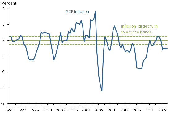
Source: Bureau of Economic Analysis and authors’ calculations.
For these deviations, Figure 2 shows the number of quarters it took for inflation to return to this band when it was outside (blue line). Every time inflation moves outside the band, the realized horizon increases and then decreases by one every quarter until inflation moves back within the band.
Figure 2
Realized and expected horizons for return to inflation bands
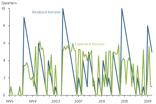
Source: Bureau of Economic Analysis and authors’ calculations.
To generate a forecast of inflation each quarter, we use a hybrid New Keynesian macroeconomic model based on Linde (2005). The model-predicted paths imply the expected horizons needed for inflation to move back within the band, displayed by the green line in Figure 2. As opposed to the realized horizon, which simply counts down until inflation is back within the band, the expected horizon varies based upon the evolving state of the economy. For example, the expected horizon can either increase or remain the same over time if economic shocks lead to inflation persistently remaining outside the band. In our proposed framework, the comparison between the expected horizon and the realized horizon can then be used to evaluate monetary policy.
Evaluating monetary policy
Figure 3 shows the difference between the two series shown in Figure 2, the model-implied expected time horizon and the realized horizon under our baseline policy (blue line). If the realized horizon always exactly met the expected horizon, the two would be the same and the series would always be zero. In practice, however, the realized and expected horizons differ, with deviations on both the positive and negative side. Positive deviations indicate inflation was brought back to within the range earlier than expected, and negative deviations indicate it was later than expected.
Figure 3
Comparing stated and realized horizons in scenario
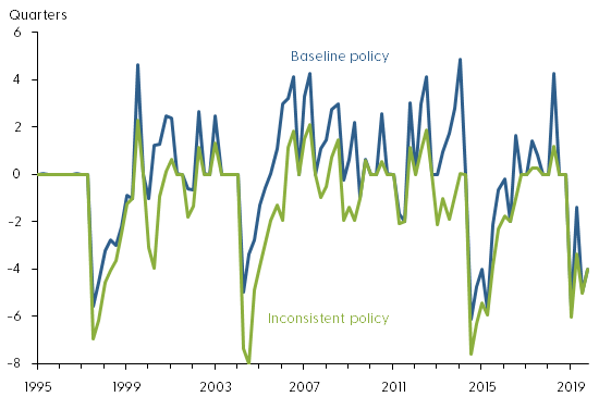
Source: Authors’ calculations.
The fact that realized horizons differ from expected horizons is not surprising and would not by itself indicate any shortcomings of policy. In general, with shocks hitting the economy and constantly generating fluctuations in inflation, we would expect deviations like those seen in Figure 3 to be the rule rather than the exception. For the most part, deviations from shocks would tend to be small and symmetric—small because only larger or repeated shocks would generate large deviations, and symmetric because typically the expected horizon could be missed due to either positive or negative shocks to inflation. Deviations may occasionally be larger or more systematic due to specific developments, such as the large negative deviation starting in 2014 that was associated with oil price declines and a recession-like slowdown in investment (Foerster 2017).
One way to assess monetary policy is by examining whether there is a systematic bias in the deviations. This could indicate when monetary policy actions differ from previously stated aims. In our baseline results, we find no bias in this history scenario. But to illustrate how a failure to follow through on policy would look to the public, Figure 3 also shows an “inconsistent policy” scenario (green line), where the central bank communicates a stronger response of interest rates compared to the baseline policy and thus a relatively shorter expected horizon for inflation to return within the band. However, when the time comes to implement such a plan, the central bank does not follow through with a strong policy response and opts for a more accommodative policy rate. In this way, the country’s stated plans are inconsistent with how it sets policy.
Under the inconsistent policy, the expected horizons are shorter than under the baseline policy, reflecting the desire to bring inflation back to the band particularly fast.
However, compared to the baseline case, the inconsistent policy shows up as a larger average difference between the expected horizon and the realized one. In Figure 3, the average deviation over the whole sample is close to zero in the baseline policy, reflecting that the realized horizons are consistent with the stated policy intent. In contrast, the average deviation for the inconsistent policy alternative is more than four months. Thus, using horizons can help assess whether monetary policy is following through on its previous intentions and statements.
While the focus of this Letter has been on strict inflation targeting, using bands and horizons to assess performance can be extended to other targets of monetary policy such as the output gap, output growth, or the unemployment rate. For example, a central bank that targets inflation and unemployment could add a projected horizon for hitting a given unemployment rate and then compare the realized horizon with the expected one.
Conclusion
Inflation-targeting central banks differ in how they conduct policy and how they measure success. We propose a framework that uses inflation bands around a point target, coupled with communications of expected horizons for bringing inflation back to the band when it moves outside. This approach is straightforward to communicate to the public and generates a measure that can be useful for assessing monetary policy effectiveness for inflation and could be extended to evaluate other central bank goals.
Troy Davig
Symmetry Investments
Andrew Foerster
Senior Research Advisor, Economic Research Department, Federal Reserve Bank of San Francisco
References
Davig, Troy, and Andrew Foerster. 2023. “Communicating Monetary Policy Rules.” European Economic Review 151(104290, January).
Foerster, Andrew. 2017. “Characterizing the 2014–16 Slowdown in Investment.” FRB Kansas City Macro Bulletin, December 20.
Linde, Jesper. 2005. “Estimating New-Keynesian Phillips Curves: A Full Information Maximum Likelihood Approach.” Journal of Monetary Economics 52(6), pp. 1,135–1,149.
McDermott, John, and Rebecca Williams. 2018. “Inflation Targeting in New Zealand: An Experience in Evolution.” In Central Bank Frameworks: Evolution or Revolution?, eds. John Simon and Maxwell Sutton. Sydney: Reserve Bank of Australia, pp. 7–23.
Walsh, Carl. 2015. “Goals and Rules in Central Bank Design.” International Journal of Central Banking 11(S1), pp. 295–352.
Opinions expressed in FRBSF Economic Letter do not necessarily reflect the views of the management of the Federal Reserve Bank of San Francisco or of the Board of Governors of the Federal Reserve System. This publication is edited by Anita Todd and Karen Barnes. Permission to reprint portions of articles or whole articles must be obtained in writing. Please send editorial comments and requests for reprint permission to research.library@sf.frb.org