
Labor market conditions are similar in regions that are near each other. This is called positive spatial correlation. Analyzing county-level data from 1990 to 2024 shows that commuting flows may contribute to strong spatial correlation in employment growth. Spatial correlation appears to have strengthened since the 1990s, at the same time as more workers were commuting across county lines. As these connections grow through commuting flows, both favorable and challenging conditions in local economies may become more likely to spread farther than in the past.
Regions that are geographically close are much more likely to share similar economic conditions than regions that are farther apart. Put in economic terms, regional conditions tend to have positive spatial correlation. This reflects that economic activity seldom stops or starts abruptly at borders on a map. Rather, characteristics that influence local economies—such as population density, demographics, and industry composition—show smooth and gradual variation across nearby regions.
In this Economic Letter, we document spatial correlation in labor market conditions by looking at county-level employment growth. We find that labor market conditions exhibit positive spatial correlation, as expected and consistent with past work (see, for example, Fogli, Hill, and Perri 2013). The strength of that relationship appears to have increased over time. We also find that commuting patterns can contribute to spatial correlation, which is consistent with existing research (see Patacchini and Zenou 2007, Monte, Redding, and Rossi-Hansberg 2018, and Bartik 2024). The rise in spatial correlation aligns with a rise in cross-county commuting. A basic simulation from 1990 to 2024 using our results suggests that employment estimates that include spatial correlation grow about 2.6% more than employment estimates without.
Understanding these patterns and their variation over time can help explain how changes in one region may affect conditions in other nearby regions. With more Americans living farther from work, our results suggest that economic ties could strengthen between ever-wider areas, spreading localized economic shocks farther now than in the past.
Spatial correlation in labor market conditions
Labor market conditions in geographically close areas are similar. For example, employment growth in San Francisco County, home to the Federal Reserve 12th District’s head office, generally follows patterns that are more similar to those in the surrounding Bay Area counties than in other highly populated California counties. That is, the correlation is higher between San Francisco County and neighboring counties than with non-neighboring counties. Moreover, employment growth in San Francisco County is more strongly correlated with employment growth in California overall than with employment growth in other states.
Figure 1 demonstrates this pattern using the 12-month percent change in employment for each county. Though there is substantial variation, there are clusters of counties with higher growth rates and clusters of counties with lower growth rates. This is a demonstration of positive spatial correlation: Like clusters with like.
Figure 1
Employment growth by county, December 2023
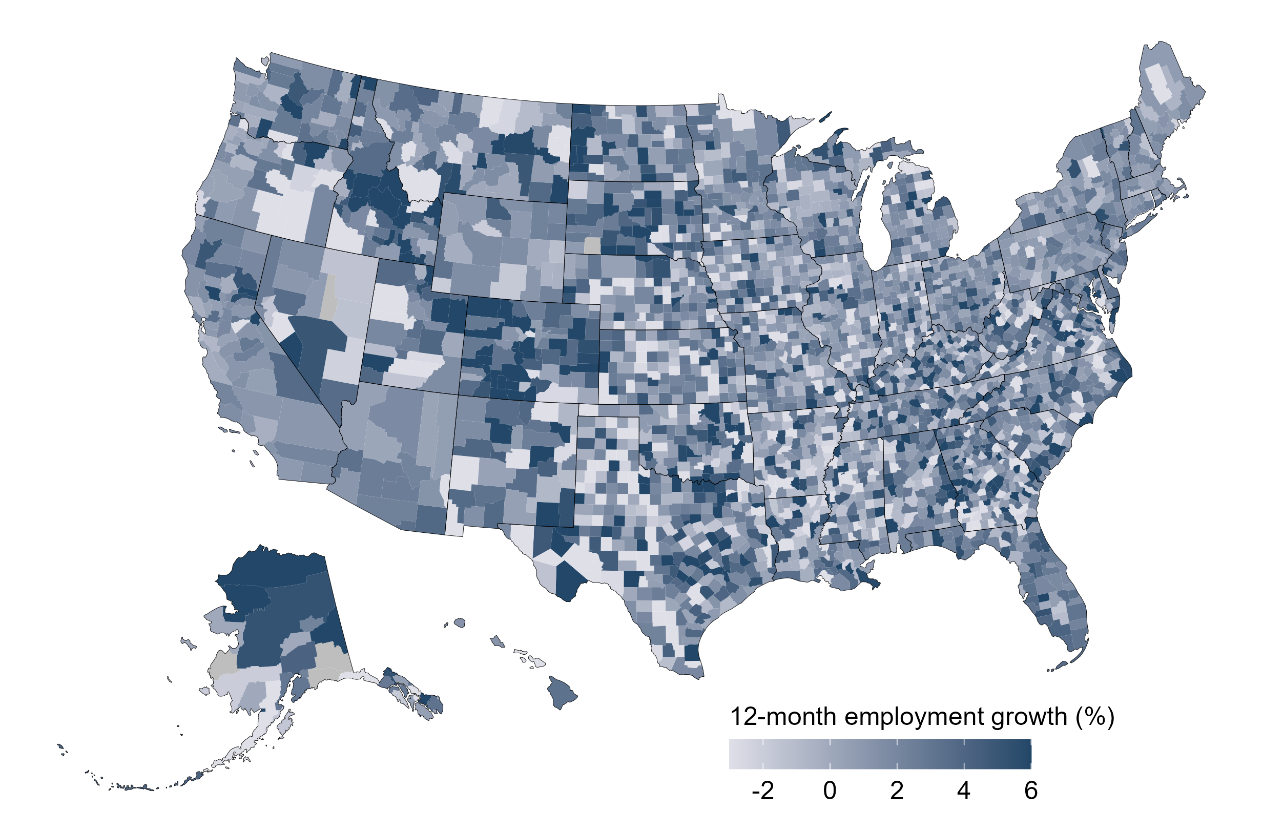
Source: Authors’ calculations from the U.S. Bureau of Labor Statistics’ Quarterly Census of Employment and Wages (QCEW).
To quantify the cross-county patterns from the map, we calculate the correlation between 12-month employment growth rates for each pair of counties. Then, we group county pairs based on the geographic distance between them and calculate the average correlation for counties in each group.
As Figure 2 shows, the average correlation is generally higher at smaller distances than at larger distances. While the figure summarizes correlations between counties up to 1,200 miles apart, it is worth noting that the correlation rises somewhat at much larger distances. The reason is that these higher distance comparisons include county pairs with large cities, including those on opposite coasts. Because of similarities in demographic and industry composition and other characteristics, employment growth tends to be highly correlated in these large cities despite the geographic distance between them. For example, the correlation between New York County and Los Angeles County is about 0.85, even though they are over 2,400 miles apart.
Figure 2
County employment growth correlation by distance
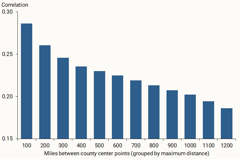
Source: Authors’ calculations from QCEW and National Bureau of Economic Research County Distance Database.
This comparison illustrates a general point that, while geographic distance is often used to estimate spatial correlation, distance itself is not the underlying reason for spatial correlation. The ultimate mechanisms are based on economic linkages, such as the flow of goods through trade and of people through commuting and migration. Counties that are more geographically distant may actually be much “closer” when measured by economic activity.
Commuting patterns as a measure of proximity
Our study focuses on the basic idea that commuters could spread changes in economic conditions from one area to another because they work in one place but live somewhere else. To illustrate this, say that monthly employment growth is strong in San Francisco County. Some people hired there are likely to live elsewhere, for example across the bay in Alameda County, and will spend money there. This additional spending increases demand and encourages employment growth in Alameda County, increasing the spatial correlation in economic activity.
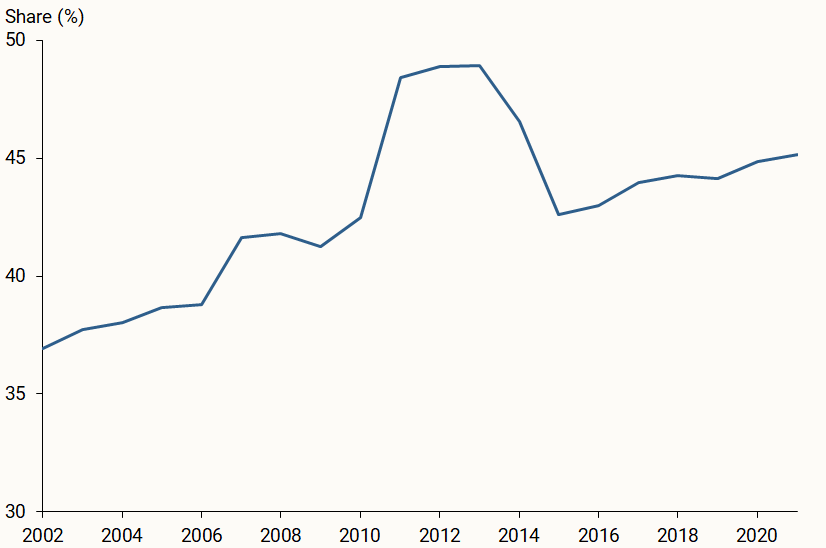
We first examine the amount of cross-county commuting. The U.S. Census Bureau’s Longitudinal Employer-Household Dynamics Origin-Destination Employment Statistics (LODES) program provides counts of jobs by workers’ county of employment and residence. The data come from administrative records and are available annually from 2002 through 2021. We use these data to estimate the share of jobs filled by workers who do not live in the same county in which their job is based. Although it does not perfectly capture the commuting share, the out-of-county job share offers a suitable proxy for commuting, and we refer to it as such for simplicity. One limitation is that LODES data may overstate cross-county commuting. For example, the job of an Alameda County resident working at an Alameda County branch may sometimes be recorded as a job at the company’s headquarters, say in New York County. This would create a nonexistent cross-county commuting flow in the data. To account for this, we omit jobs that make up a very small share of a county’s out-of-county jobs.
Figure 3 shows that the out-of-county job share is relatively high and has generally grown over time. Longer commutes, tighter housing supplies in areas where jobs are concentrated, and, to some degree, trends in remote work likely contributed to the increase. The rise and fall around the 2007–09 recession may have been driven by people having to take jobs farther from home when the labor market was weaker and then finding a job closer to home as the labor market recovered. The key message is that cross-county commuting is prevalent and has risen over time, indicating that commuting could create more meaningful linkages between county economies.
Figure 3
Share of jobs filled by residents of other counties
To quantify how much labor market conditions in counties linked by commuting flows influence each other, we first need a measure of labor market conditions in each county. We use monthly data from the Quarterly Census of Employment and Wages (QCEW) from 1990 to 2024. To abstract from national trends, we measure our county-level data relative to their national equivalents. Following past research, we construct the component of monthly employment growth that is due solely to a county’s industry composition. This helps capture labor market conditions that are specific to a given county rather than conditions that reflect broader regional trends.
Second, we need a way to summarize our measure of labor market conditions across a county’s commuting neighbors. We accomplish this with a weighted average. The LODES data allow us to determine the set of neighboring commuting counties to use for calculating the average. The data also tell us the commuting shares between counties, which we use to weight each neighbor’s growth. We refer to the resulting weighted average as neighbor employment growth.
Quantifying how much neighboring county conditions matter
We use regression analysis to estimate the relationship between a county’s monthly employment growth and labor market conditions among its neighbors, both relative to the national average. We account for recent past employment growth in the county and its neighbors, time trends, seasonality, time-invariant county factors, and monthly wage growth.
Figure 4 shows the average relationship between county employment growth and our neighbor employment growth measure by decade, along with 95% confidence bands. The results confirm the spatial correlation observed in Figures 1 and 2. For example, if average neighbor employment growth is 1 percentage point higher, county employment growth will typically be 0.5 percentage point higher according to the current estimated relationship (rightmost bar). Comparing across decades, the relationship between counties and their neighbors appears to have strengthened over time. The estimates rise from about 0.2 in the 1990s to about 0.5 in the first half of the 2020s. The increase coincides with the rise in commuting shares from Figure 3, although the difference between the estimates is not statistically significant.
Figure 4
Employment growth response to neighbor growth
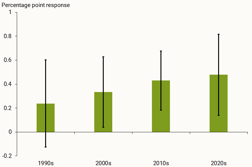
Source: Authors’ calculations from QCEW and LODES data.
To the extent that the neighbor measure captures unexpected changes in employment growth, or labor demand shocks, our results indicate that shocks can spread from one county to another. Furthermore, the full impact of such shocks could take some time to appear in neighboring counties; regression coefficients on some lags of the neighbor variable are positive and statistically significant, which is consistent with shock propagation over time (not shown). We interpret these results cautiously because the lagged coefficients fluctuate; however, they are in line with some prior research on shock propagation along commuting linkages, including Patacchini and Zenou (2007), Fogli, Hill, and Perri (2013), and Monte, Redding, and Rossi-Hansberg (2018).
An implication of our findings is that linkages between counties could amplify business cycle fluctuations in employment growth. A basic application of our model suggests that this occurs to some degree, particularly over long economic expansions. We use our model to simulate total employment starting in 1990, with and without the effects of neighboring counties. By the end of our sample period in 2024, employment estimated with the neighbor effects is about 2.6% higher than estimates without—representing about 4 million jobs. The gap between the estimates generally widens during economic expansions and shrinks slightly during recessions. This is consistent with prior research finding that linkages can amplify business cycle swings in labor market conditions (Fogli, Hill, and Perri 2013).
Conclusion
This Economic Letter documents a robust relationship between employment growth in nearby counties, known as positive spatial correlation. The strength of this relationship appears to have increased somewhat over time. Results suggest that commuting flows are part of the underlying mechanisms that transmit economic conditions between counties. As increasing numbers of workers travel farther to work, this could hasten the spread of initially localized changes in economic conditions across regions.
References
Bartik, Timothy J. 2024. “Local Labor Markets Should Be Redefined: New Definitions Based on Estimated Demand-Shock Spillovers.” Upjohn Institute Working Paper 24-407.
Fogli, Alessandra, Enoch Hill, and Fabrizio Perri. 2013. “The Geography of the Great Recession.” In NBER International Seminar on Macroeconomics 9(1), pp. 305–331. Chicago, IL: University of Chicago Press.
Monte, Ferdinando, Stephen J. Redding, and Esteban Rossi-Hansberg. 2018. “Commuting, Migration, and Local Employment Elasticities.” American Economic Review 108(12), pp. 3,855–3,890.
Patacchini, Eleonora, and Yves Zenou. 2007. “Spatial Dependence in Local Unemployment Rates.” Journal of Economic Geography 7(2), pp. 169–191.
Opinions expressed in FRBSF Economic Letter do not necessarily reflect the views of the management of the Federal Reserve Bank of San Francisco or of the Board of Governors of the Federal Reserve System. This publication is edited by Anita Todd and Karen Barnes. Permission to reprint portions of articles or whole articles must be obtained in writing. Please send editorial comments and requests for reprint permission to research.library@sf.frb.org