An accurate measure of economic slack is key to properly calibrate monetary policy. Two traditional gauges of slack have become harder to interpret since the Great Recession: the gap between output and its potential level, and the deviation of the unemployment rate from its natural rate. As a consequence, conventional policy rules based on these measures of slack generate wide-ranging policy rate recommendations. This variability highlights one of the challenges policymakers currently face.
It would be a mistake to characterize the Great Recession as simply a run-of-the-mill economic downturn, only larger in magnitude. In the post-World War II era the United States experienced both deep recessions and episodes of financial turmoil, but not since the Great Depression had the U.S. economy suffered both simultaneously. The degree of economic dislocation has been considerable, greatly altering the long-term structure of the economy and the outlook.
Economists are still grappling with this new economic order and how to refine their thinking. Not surprisingly, implementing policy in such an uncertain economic environment has been specially challenging. This Economic Letter examines how this new environment has made traditional measures of economic performance harder to interpret. The tool we use to communicate these policy challenges is the well-known Taylor rule.
This is the first in a two-part series. The second (Bosler, Daly, and Nechio 2014) details mixed signals from the labor market.
Large revisions to potential output
The deviation of real GDP from its potential level has long been regarded as a standard measure of economic slack. When the economy grows faster than its potential, the effects are widespread: Overtime hours increase for workers, capital utilization rates go up for businesses, and inflation pressures mount for consumers. Not surprisingly, the difference between real GDP and its potential level, known as the output gap, is closely scrutinized by policymakers. Although potential GDP is not directly observable, the Congressional Budget Office (CBO) regularly publishes an estimate of its value.
Data on both real GDP and potential GDP go through a number of revisions. Data on real GDP come from the National Income and Product Accounts (NIPA) published by the Bureau of Economic Analysis. The NIPA relies on a wide variety of data that differ in quality, coverage, and availability. Initial GDP estimates rely mostly on smaller-scale surveys, which are available reasonably quickly. Over time, survey data are replaced with large-scale census data, which are more exhaustive but take longer to collect.
Figure 1
Revisions to potential GDP
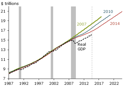
Sources: BEA and CBO, chained 2009 dollars.
By contrast, potential GDP estimates are revised less frequently. Moreover, past revisions have usually been small so that even initial estimates about future values have been reliable. Potential GDP had moved slowly enough that the CBO releases yearly updates together with 10-year projections. However, the Great Recession eradicated this stability and has vividly demonstrated how quickly estimates of potential GDP can change in times of economic tumult. Between 2007 and 2014, the CBO revised its projection of real potential GDP for the first quarter of 2014 downward by almost 8%. Figure 1 depicts the CBO’s 10-year projections of potential GDP from 2007, 2010, and 2014 alongside the path of real GDP for context.
A primer on the Taylor rule
How significant are these revisions of potential GDP, and how do they affect a policymaker’s assessment of current economic conditions? This is difficult to answer considering only the data in Figure 1. We can get a more complete picture by examining how revisions to potential GDP affect the policy recommendations one would derive from a textbook policy rule such as the Taylor (1993) rule. This benchmark is designed with price and output stability in mind. The rule incorporates two essential elements to handle inflation’s deviation from its targeted level and output’s deviation from its potential level. If inflation is at its target and the economy is growing on par with its potential, these two penalty terms vanish and the policy rate equals the nominal equilibrium rate of interest.
There are numerous modifications to the original rule in Taylor (1993). Taylor (1999), Rudebusch and Svensson (1999), and Coibion and Gorodnichenko (2005) provide good surveys. These modifications run the gamut, from using forecasts rather than current values of inflation and output to adding a smoothing term to capture the incremental way the policy rate is typically adjusted. The version we use here was discussed in Taylor (1999) and has since gained wide acceptance as a natural benchmark.
According to this version of the rule, the policy rate can be expressed as follows:
Policy rate = 1.25 + (1.5 × Inflation) + Output gap.
We measure inflation using the personal consumption expenditures price index (PCEPI) excluding food and energy. This measure is commonly referred to as core PCE inflation. Although the Federal Reserve is ultimately interested in ensuring that headline inflation remains stable, core inflation is significantly less volatile and therefore offers a more reliable measure (see Bernanke 2007). We measure the output gap using the percentage difference between real GDP and its potential. The intercept in this rule is based on an estimate of the natural rate of interest; our conclusions would only be reinforced if we accounted for the greater uncertainty about the natural rate of interest in the wake of the Great Recession (Leduc and Rudebusch 2014).
Figure 2
Taylor rules by potential GDP estimates
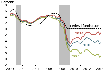
Sources: BEA, CBO, and authors’ calculations.
Potential GDP and the Taylor rule
Figure 2 depicts three different policy rate paths using the 2007, 2010, and 2014 vintages of the CBO’s potential GDP plotted against the actual target for the federal funds rate, the U.S. policy rate. The estimated policy rates track the federal funds rate and each other fairly closely until the end of 2008, when the federal funds rate hits the zero lower bound and the three alternative policy paths begin to diverge significantly.
This divergence comes from the sequential revisions to potential GDP. Mechanically, the recommended policy rate increases as the output gap diminishes. With time and more current data, a more accurate picture of the recession and how it had affected potential GDP emerged. Notice that the 2007 and 2010 estimates of the output gap are so large and negative that the benchmark Taylor rule suggests the policy rate should be negative for most of the period since 2008. Based on the 2007 estimates of potential GDP and the value of actual GDP today, the Taylor rule would recommend a policy rate of –8.7%. This striking number underscores the importance of the revisions to potential GDP.
From output gap to unemployment gap with Okun’s law
A popular alternative for assessing slack in the economy is to use the unemployment gap, the gap between the unemployment rate and its natural rate. This alternative gap measure offers two main advantages for policymakers. First, unemployment data are available monthly as opposed to quarterly for GDP data. Second, unemployment numbers offer a more direct discussion of the one of the Fed’s explicit mandates, full employment. It is natural to ask then whether the unemployment gap provides a cleaner measure of economic slack than the output gap and to determine how these measures are related.
Okun’s law is a popular rule of thumb that relates changes in the unemployment rate to GDP growth at an approximate two-to-one ratio. However, underlying this empirical regularity are important economic mechanisms that justify the result and illuminate the link between the output and unemployment gaps. For example, when businesses face declining demand, they reduce production using a blend of fewer hours per worker, reduced staffing levels, decreased capital utilization levels, and changes in technology. Historically, Okun’s law has been a remarkably stable relationship, but the Great Recession has muddied the waters, as discussed in Daly, et al. (2014).
Using Okun’s law, the Taylor rule can easily be rewritten to incorporate an unemployment gap in place of the output gap:
Policy rate = 1.25 + (1.5 × Inflation) – (2 × Unemployment gap).
The unemployment gap is measured as the percentage point difference between the unemployment rate and the non-accelerating inflation rate of unemployment, or NAIRU. The NAIRU, just like potential GDP, is not directly measurable. However, the CBO regularly releases estimates of its value. These estimates are closely linked to those of potential GDP and include several adjustment factors, for example, based on the potential size of the labor force or potential labor force productivity. The version of the Taylor rule that uses the unemployment gap is discussed in Rudebusch (2010).
Figure 3
Two Taylor rules
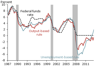
Sources: BEA, CBO, BLS, and authors’ calculations.
Before 2008, the policy rates recommended by the output and unemployment gap versions of the benchmark Taylor rule remained within a few fractions of a percentage point of each other and reasonably close to what the federal funds rate turned out to be, as illustrated in Figure 3. Note that we use the most up-to-date measures of potential GDP and the NAIRU to abstract from the variation induced by revisions and focus exclusively on the different signals provided by each gap measure.
Policy recommendations diverged considerably once the Great Recession was under way. If we ignore the zero lower bound on nominal interest rates, the unemployment gap version of the Taylor rule called for policy to be set about 3 percentage points lower than the output gap version would have suggested throughout 2010. The differences between the two narrowed over the next few years, and by 2012 they appeared to be as close as in the past.
Recently, however, the unemployment rate has been gradually improving, whereas economic performance, as measured by real GDP growth, has remained lackluster. As a result the difference in the suggested policy rates has flipped: the unemployment gap version of the Taylor rule now calls for policy to be about 2 percentage points higher than the output gap version. Once again, it appears that Okun’s law and the margins firms use to adjust to the new economic environment have temporarily diverged from normal. Conflicting signals from labor markets may shed some light on this recent divergence, an issue that will be explored in the second part of this series (Bosler, Daly, and Nechio 2014).
Conclusion
Determining whether the economy is overheating or underperforming is critical for monetary policy. Policymakers cannot simply rely on one indicator to make this judgment. This Letter has shown that in times of economic turmoil it is especially difficult to get a clear read on the economy’s potential, and different indicators can generate conflicting signals. Our analysis highlights the difficulties of using the Taylor rule as a practical guide to implementing monetary policy in real time.
Early Elias and Helen Irvin are research associates in the Economic Research Department of the Federal Reserve Bank of San Francisco.
Òscar Jordà is a senior research advisor in the Economic Research Department of the Federal Reserve Bank of San Francisco.
References
Bernanke, Ben. 2007. “Semiannual Monetary Policy Report to the Congress.” July 18.
Bosler, Canyon, Mary C. Daly, and Fernanda Nechio. 2014. “Mixed Signals: Labor Markets and Monetary Policy.” FRBSF Economic Letter 2014-36 (December 1).
Coibion, Olivier, and Yuriy Gorodnichenko. 2012. “Why Are Target Interest Rate Changes So Persistent?” American Economic Journal: Macroeconomics 4(4), pp. 126–162.
Daly, Mary, John Fernald, Òscar Jordà, and Fernanda Nechio. 2014. “Interpreting Deviations from Okun’s Law.” FRBSF Economic Letter 2014-12 (April 21).
Leduc, Sylvain, and Glenn D. Rudebusch. 2014. “Does Slower Growth Imply Lower Interest Rates?” FRBSF Economic Letter 2014-33 (November 10).
Rudebusch, Glenn D. 2010. “The Fed’s Exit Strategy for Monetary Policy.” FRBSF Economic Letter 2010-18 (June 14).
Rudebusch, Glenn D. and Lars E.O. Svensson. 1999. “Policy Rules for Inflation Targeting.” In Monetary Policy Rules, ed. John Taylor. Chicago: University of Chicago Press.
Taylor, John B. 1993. “Discretion versus Policy Rules in Practice.” Carnegie-Rochester Conference Series on Public Policy 39, pp. 195–214.
Taylor, John B. 1999. “The Robustness and Efficiency of Monetary Policy Rules as Guidelines for Interest Rate Setting by the European Central Bank.” Journal of Monetary Economics 43(3), pp. 655–679.
Opinions expressed in FRBSF Economic Letter do not necessarily reflect the views of the management of the Federal Reserve Bank of San Francisco or of the Board of Governors of the Federal Reserve System. This publication is edited by Anita Todd and Karen Barnes. Permission to reprint portions of articles or whole articles must be obtained in writing. Please send editorial comments and requests for reprint permission to research.library@sf.frb.org