
Interest rates are inherently difficult to predict, and the simple random walk benchmark has proven hard to beat. But macroeconomics can help, because the long-run trend in interest rates is driven by the trend in inflation and the equilibrium real interest rate. When forecasting rates several years into the future, substantial gains are possible by predicting that the gap between current interest rates and this long-run trend will close with increasing forecast horizon. This evidence suggests that accounting for macroeconomic trends is important for understanding, modeling, and forecasting interest rates.
Anticipating future changes in interest rates is an obvious concern for investors. It’s also important for policymakers, professional forecasters, and academics because interest rates affect household finances, business funding costs, government debt, and ultimately the health of the overall economy. Unfortunately interest rates, much like the stock market, are very hard to predict. Indeed, the simple forecast that predicts future interest rates will not change at all is hard to beat, and even sophisticated models do not consistently perform better.
Although accurate predictions are elusive for relatively short horizons—say for rates one day, one week, or even one year in the future—economic theory can improve predictions of interest rates over longer horizons. Just like the booms and busts of economic activity manifest themselves around an underlying trend of long-run economic growth, interest rates also fluctuate around a trend that is driven by slow-moving or structural forces. This Economic Letter explains how the same principles used for economic forecasts of macroeconomic variables, like output growth or inflation, can be applied to interest rates. The basic idea outlined here, with further detail and empirical evidence in Bauer and Rudebusch (2017), is that the trend underlying the evolution of interest rates is closely related to two important macroeconomic variables: the underlying trend in inflation and the equilibrium real interest rate.
Why is it so hard to forecast interest rates?
The difficulty of predicting changes in interest rates mainly arises from two features that characterize their evolution over time. First, like other financial variables, interest rates vary widely from day to day, which makes them difficult to link to economic fundamentals such as monetary or fiscal policy. This well-documented “excess volatility,” was first pointed out in Shiller (1979), and it reflects the importance of frequent changes in investor sentiment due to a never-ending stream of economic data releases and other news.
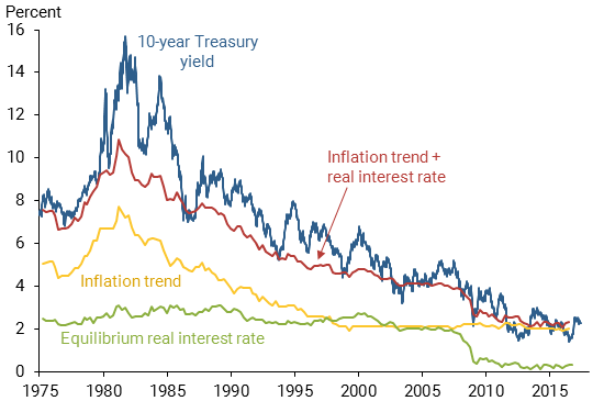
Second, as evident from 10-year Treasury yields since 1971, seen in Figure 1, interest rates have not fluctuated around a stable average level over this period. Instead of “mean reversion” around a constant average, they exhibit slow-moving trends, such as the rise during the “Great Inflation” period of the 1970s, and the long-lasting decline since then.
Figure 1
Macroeconomic trends and 10-year Treasury yield
Neither the short-run movements nor the long-run trends are easily predicted using existing models. Although a large variety of statistical and theoretical models have been developed to better understand the properties and determinants of interest rates, their forecast performance is typically disappointing. Some models forecast well over certain periods, for example, Christensen, Diebold, and Rudebusch (2011). But no forecast approach has been able to consistently improve upon the simple “random walk” model, which assumes that increases and decreases are equally likely and therefore always forecasts no change (Duffee 2013). And although a number of different variables seem to help predict interest rates in simple statistical models, such findings often turn out to be a statistical fluke due to complications arising from small sample sizes (Bauer and Hamilton 2017).
Forecasting in the presence of trends
In macroeconomics, on the other hand, a consensus has emerged that successful forecasts of economic data series like inflation or output growth require three ingredients. The first is a “nowcast,” the current value of the series which is typically an estimate due to publication lags and data revisions. The second is an estimate of the series’ long-run trend, which is the level the series is expected to settle down to after all transitory ups and downs have dissipated. The final ingredient is a stance or framework to guide how the transition from the current level to the long-run level will play out, in particular how quickly or slowly the series will return to its trend. Thus, economic forecasting generally comes down to answering three heuristic questions: Where are we now? Where are we going? And, how are we going to get there?
This conceptual framework for forecasting may be called the “gap model” due to its focus on the gap between the current level and the long-run level, as well as on how quickly this gap is closed. Importantly, the gap model recognizes that the trend component is not constant but instead shifts due to changes in the economy. In other words, the gap model does not assume that the level of the series will revert to some constant mean, but instead that the gap between the series and its trend component will revert to zero. Estimating trend components and gaps underlies most macroeconomic forecasting, and Faust and Wright (2013) recently demonstrated the gap model’s excellent performance for inflation forecasting.
The apparent downward trend in long-term interest rates evident in Figure 1 suggests that the gap model could hold some promise. Current interest rates are directly available from market data. But estimating the trend component and constructing the gap between the current level and trend appear to be more difficult, which may be why existing models for interest rates either assume a constant average level or base predictions on the current level, as in the random walk method.
Fortunately, economic theory suggests a relatively simple way to estimate the trend in interest rates, based on the insight that interest rates can be viewed as the sum of inflation expectations and inflation-adjusted, “real” interest rates. Therefore the trend in interest rates equals the sum of the trend in inflation and the trend in the real interest rate. Since inflation is ultimately determined by monetary policy, the long-run inflation trend corresponds to the perceived inflation target of the central bank. This can be estimated reasonably well from surveys. Figure 1 plots the publicly available and mostly survey-based inflation trend estimate (red line) that underlies the Federal Reserve Board’s structural model of the U.S. economy, FRB/US. For the trend in the real interest rate, also called the natural or equilibrium real interest rate, Laubach and Williams (2003) suggested a way to estimate it from macroeconomic data and popularized its use in policy analysis (see also Williams 2016). Figure 1 includes an estimate of the equilibrium real interest rate (green line) taken as the average of several popular estimates, as discussed in Bauer and Rudebusch (2017).
Figure 1 also plots the sum of these two trends (red line); this estimate of the trend component in interest rates has exhibited a very pronounced decline since the 1980s. The 10-year yield generally fluctuated near this trend, and both are currently very low in historical comparison, with important consequences for policymaking (Williams 2016). Figure 1 suggests that it may be useful to take into account the level of the trend when forecasting interest rates.
With nowcasts and trend estimates in hand, the final piece required for a practical forecast rule is an assumption about the transition of interest rates to their trend. Based on how quickly interest rates have historically reverted back to the trend, a reasonable assumption to make for this forecasting exercise is that 20% of the remaining gap is closed each quarter. But the precise speed of reversion to the trend is typically not crucial for forecasting performance (Faust and Wright 2013). Furthermore, it becomes essentially irrelevant for long-horizon forecasts, since forecasts are approximately equal to the estimated trend.
Evaluating forecast accuracy
The next step is to use historical data to evaluate how accurate this gap model for interest rates is compared with four alternative forecast methods. The goal is to forecast where the 10-year yield will be five years from the date the forecast is made; Bauer and Rudebusch (2017) have shown that forecasting other interest rates, like the five-year yield, or considering other long forecast horizons leads to similar results. The alternative methods are the no-change or random walk forecast, which predicts the current level of the interest rate will prevail in subsequent periods; the mean reversion forecast, representative of a large class of existing models, which assumes a constant mean estimated based on the data available up to the date of the forecast; a market-based forecast, which uses the implied future interest rate, the so-called forward rate, based on the current 5- and 15-year yields; and survey forecasts from the Blue Chip Financial Forecasts, which since 1988 has released long-range estimates about twice every year.
Figure 2 shows the average absolute forecast errors as a measure of forecast accuracy for the five different forecasting methods, both for a long period, 1971–2016, and a short one, 1988–2016, over which the Blue Chip forecasts are available. The gap model produces forecasts that on average are much more accurate than those from the other methods over both sample periods. For example, over the shorter sample the absolute forecast error from the gap model averaged only 0.8 percentage points, while the error from the Blue Chip forecasts averaged 1.9 percentage points.
Figure 2
Forecast accuracy of 10-year yield estimates, 5 years ahead
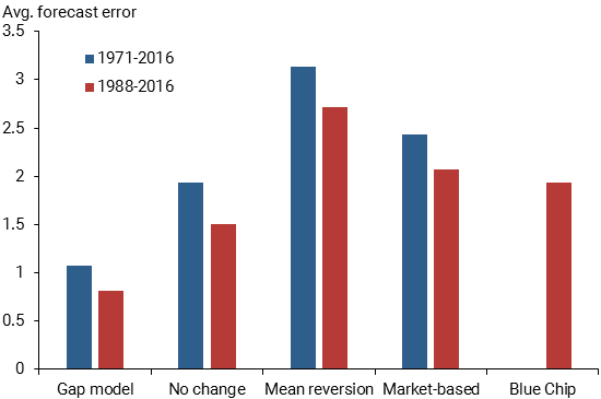
Note: Comparison of average forecast errors measured in absolute values over two sample periods.
These estimates of forecast accuracy are necessarily imprecise because the sample is quite small: Even in the full sample there are relatively few five-year forecast horizons that don’t overlap. However, despite this small sample size, the differences are statistically significant (Bauer and Rudebusch 2017).
Although I try to use only data available to forecasters at the time they issued their projections, it is difficult to completely avoid the benefit of hindsight, that is, to construct truly real-time forecasts. In particular, the models for the equilibrium real rate are estimated using the full sample of revised macroeconomic data. However, Laubach and Williams (2016) show that real-time estimates of the equilibrium real rate exhibit patterns very similar to the baseline estimates.
Conclusion
Evidence in this Letter suggests that accounting for the underlying macroeconomic trends in interest rates can substantially improve the accuracy of interest rate forecasts. It is important to bridge the gap in two different ways when forecasting interest rates. First, it is beneficial to focus on the gap between the interest rate and its underlying long-run trend. Second, macroeconomic estimates are necessary to gauge this underlying trend in interest rates, so this approach also requires bridging the gap between macroeconomics and finance.
These results are relevant not only to forecasting but also to modeling and understanding interest rates more generally. It is crucially important to account for shifts in macroeconomic trends when estimating risk premiums in bond markets, modeling how fundamental drivers such as economic growth and monetary policy affect the yield curve, and for understanding the historical evolution of interest rates over the long run.
Michael D. Bauer is a research advisor in the Economic Research Department of the Federal Reserve Bank of San Francisco.
References
Bauer, Michael D., and Glenn D. Rudebusch. 2017. “Interest Rates Under Falling Stars.” FRB San Francisco Working Paper 2017-16.
Bauer, Michael D., and James D. Hamilton. 2017. “Do Macro Variables Help Forecast Interest Rates?” FRBSF Economic Letter 2016-20 (June 27).
Christensen, Jens H.E., Francis X. Diebold, and Glenn D. Rudebusch. 2011. “The Affine Arbitrage-Free Class of Nelson-Siegel Term Structure Models.” Journal of Econometrics 164.
Duffee, Gregory. 2013. “Forecasting Interest Rates.” Chapter 7 in Handbook of Economic Forecasting, volume 2A, edited by Graham Elliott and Allan Timmermann. Amsterdam: Elsevier, pp. 385–426.
Faust, Jon, and Jonathan H. Wright. 2013. “Forecasting Inflation.” Chapter 1 in Handbook of Economic Forecasting, volume 2A, edited by Graham Elliott and Allan Timmermann. Amsterdam: Elsevier, pp. 2–56.
Laubach, Thomas, and John C. Williams. 2003. “Measuring the Natural Rate of Interest.” Review of Economics and Statistics 85(4), pp. 1,063–1,070.
Laubach, Thomas, and John C. Williams. 2016. “Measuring the Natural Rate of Interest Redux.” Business Economics 51(2).
Shiller, Robert J. 1979. “The Volatility of Long-Term Interest Rates and Expectations Models of the Term Structure.” Journal of Political Economy 87(6, December).
Williams, John C. 2016. “Monetary Policy in a Low R-star World.” FRBSF Economic Letter 2016-23 (August 15).
Opinions expressed in FRBSF Economic Letter do not necessarily reflect the views of the management of the Federal Reserve Bank of San Francisco or of the Board of Governors of the Federal Reserve System. This publication is edited by Anita Todd and Karen Barnes. Permission to reprint portions of articles or whole articles must be obtained in writing. Please send editorial comments and requests for reprint permission to research.library@sf.frb.org